Updated 04-Jan-2016 to fix a problem with the maze image that was causing an incorrect result for the cheating maze solver.

My 18-Nov-2015 post showed some of the basics of the new graph theory functionality in MATLAB R2015b. I followed that up last week with a post about my image-based graphs submission to the File Exchange.

Today I want to show you a Cheating Maze Solver based on image graphs with weighted edges.

Contents

Solving a Maze Using Shortest Path

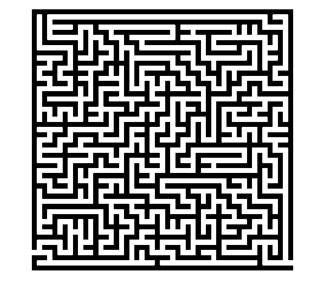
Let's start with a maze solver that doesn't cheat. Here's the maze we'll be tackling:

url = 'https://blogs.mathworks.com/steve/files/maze-51x51.png';
maze = imread(url);
maze = maze >= 128;
imshow(maze)

The first step is to construct a graph from the binary image. The nodes of the graph will be the foreground pixels, which are the paths of the maze. (The background pixels form the maze walls.)

maze_graph = binaryImageGraph(maze)

maze_graph = 

  graph with properties:

    Edges: [515967x2 table]
    Nodes: [138674x3 table]

Notice that binaryImageGraph automatically added weights to the graph edges:

maze_graph.Edges(1:5,:)

ans = 

    EndNodes    Weight
    ________    ______

    1     2          1
    1    12          1
    1    13     1.4142
    2     3          1
    2    12     1.4142

These weights are the Euclidean distances between the centers of the neighboring foreground pixels.

The start and finish coordinates for the maze are (1,496) and (533,518), which we can use to find the corresponding graph nodes.

start_node = find((maze_graph.Nodes.x == 1) & (maze_graph.Nodes.y == 496));
finish_node = find((maze_graph.Nodes.x == 533) & (maze_graph.Nodes.y == 518));

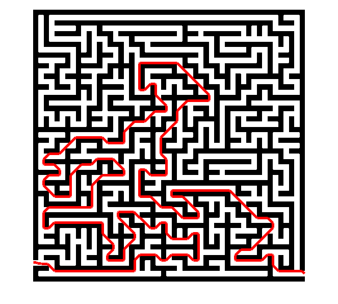
Now we just call shortestpath to find our way from the start node to the finish node. The function shortestpath returns a list of graph node indices.

p = shortestpath(maze_graph,start_node,finish_node);
p(1:5)

ans =

     5    16    27    38    49

These values can be used to index into the Nodes table of the graph.

maze_graph.Nodes(p(1:5),:)

ans = 

    x     y     PixelIndex
    _    ___    __________

    1    496     496      
    2    496    1029      
    3    496    1562      
    4    496    2095      
    5    496    2628      

Notice that the graph's node table contains the x- and y- coordinates of the corresponding image pixels. The binaryImageGraph function automatically put that auxiliary information into the graph. We can use it now to plot the shortest path.

imshow(maze)
hold on
plot(maze_graph.Nodes.x(p),maze_graph.Nodes.y(p),'r','LineWidth',5)
hold off

A Cheating Maze Solver

Now let's solve the maze by allowing the solution to tunnel through walls. To do that, we need a graph that includes foregound and background pixels, not just foreground pixels. So we build the graph using imageGraph instead of binaryImageGraph.

maze_graph2 = imageGraph(size(maze));

For any edge that touches a wall (a background pixel), let's assign a tunneling "penalty" by upping the edge weight to 100.

tunneling_penalty = 100;
touches_wall = any(~maze(maze_graph2.Edges.EndNodes),2);
maze_graph2.Edges.Weight(touches_wall) = tunneling_penalty;

This new graph has a different number of nodes, so we need to recompute the starting and finishing node numbers.

start_node = find((maze_graph2.Nodes.x == 1) & (maze_graph2.Nodes.y == 496));
finish_node = find((maze_graph2.Nodes.x == 533) & (maze_graph2.Nodes.y == 518));

Now we're ready to compute the cheating path.

tunneling_p = shortestpath(maze_graph2,start_node,finish_node);
tunneling_x = maze_graph2.Nodes.x(tunneling_p);
tunneling_y = maze_graph2.Nodes.y(tunneling_p);

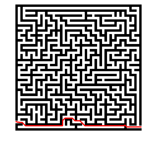
imshow(maze,'InitialMagnification','fit')
hold on
plot(tunneling_x,tunneling_y,'r','LineWidth',5)
hold off

You can see that the cheating solution tunneled through a wall in just one spot:

axis([425 535 465 535])

You can see that the shortest path jogs upwards briefly when tunneling through the wall. That's because I assigned the same edge weight penalty to diagonal neighbors as to horizontal and vertical neighbors. That means that the path length is the same for the up-and-down path as for the horizontal path. I could fix that with a somewhat more complicated edge weight computation.

Happy New Year, everyone!

Get the MATLAB code

Published with MATLAB® R2015b