
Small-Peak Suppression with the H-Maxima Transform
Last time, I introduced the idea of a regional maximum. Today, I want to add a concept that makes the regional maximum more useful: suppressing very small local maxima, possibly present only because of noise, that are are unimportant, before identifying the regional maxima. This "small peak suppression" can be accomplished using something called the h-maxima transform. The functions of interest today: imregionalmax, imhmax, imextendedmax, imregionalmin, imhmin, and imextendedmin.
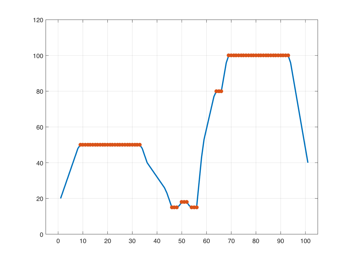
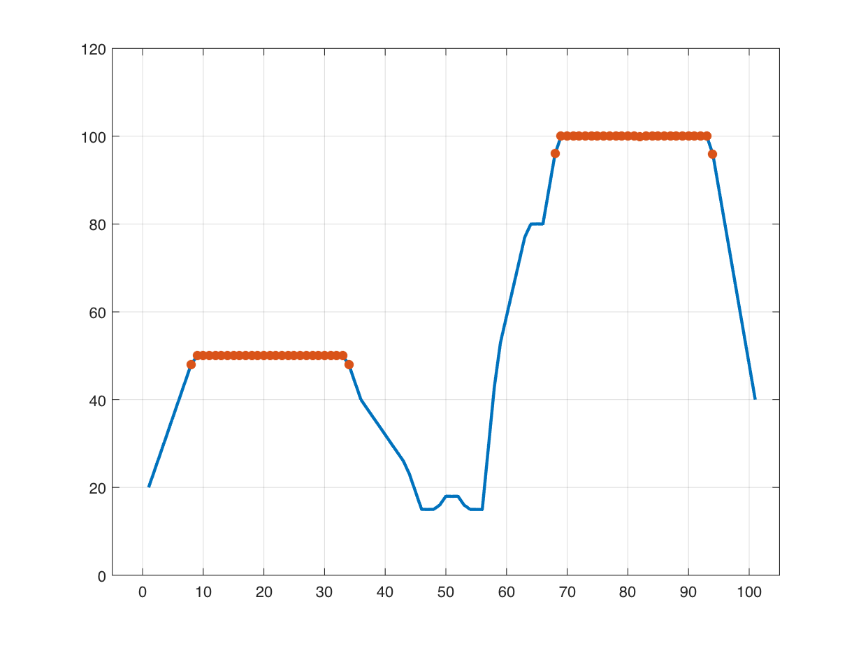
Let's get there by starting once again with the definition of regional maximum: a connected component of pixels with a constant value h, where every pixel that is neighbor to that connected component has a value that is lower than h. I'd like to elaborate on that using a one-dimensional example.
y = peaksAndPlateaus;
x = 1:length(y);
plot(x,y)
axis([-5 105 0 120])
grid on

I'll use dilation and erosion to identify curve samples that are on plateaus.
plateau_mask = (y == imdilate(y,[1 1 1])) & (y == imerode(y,[1 1 1]));
plateau_mask = imdilate(plateau_mask,[1 1 1]);
hold on
plot(x(plateau_mask),y(plateau_mask),"*")
hold off
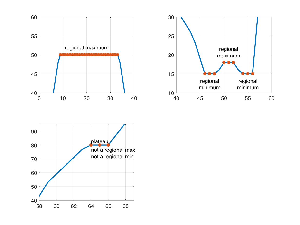
Here are some zoomed-in views that illustrate three kinds of plateaus that are of interest.
tiledlayout(2,2)
nexttile
plot(x,y)
hold on
plot(x(plateau_mask),y(plateau_mask),"*")
hold off
axis([0 40 40 60])
grid on
text(20,52,"regional maximum",HorizontalAlignment="center")
nexttile
plot(x,y)
hold on
plot(x(plateau_mask),y(plateau_mask),"*")
hold off
axis([40 60 10 30])
grid on
text(47,14,["regional" "minimum"],HorizontalAlignment = "center",...
VerticalAlignment = "top")
text(55,14,["regional" "minimum"],HorizontalAlignment = "center",...
VerticalAlignment = "top")
text(51,19,["regional" "maximum"],HorizontalAlignment = "center",...
VerticalAlignment = "bottom")
nexttile
plot(x,y)
hold on
plot(x(plateau_mask),y(plateau_mask),"*")
hold off
axis([58 69 40 95])
grid on
text(66,83,"plateau",HorizontalAlignment = "right")
text(64,79,["not a regional max" "not a regional min"],...
HorizontalAlignment = "left", VerticalAlignment = "top")
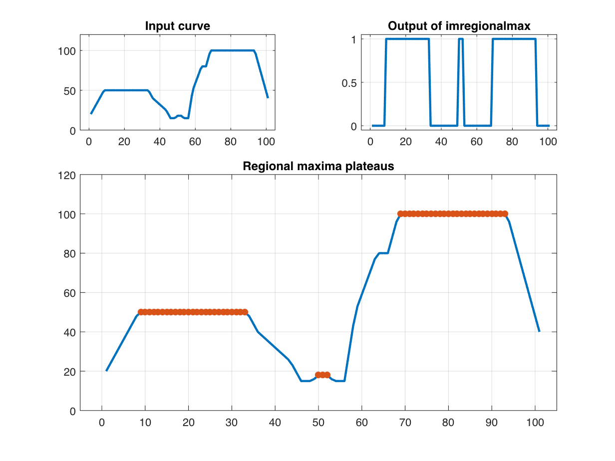
As I showed last time, the function imregionalmax identifies the location of regional maxima. These can be individual samples or pixels, or they can be plateaus. Take a look:
reg_max_mask = imregionalmax(y);
tiledlayout(3,2)
nexttile
plot(x,y)
axis([-5 105 0 120])
grid on
title("Input curve")
nexttile
plot(x,reg_max_mask)
axis([-5 105 -0.05 1.05])
grid on
title("Output of imregionalmax")
nexttile([2 2])
plot(x,y)
hold on
plot(x(reg_max_mask),y(reg_max_mask),"*")
hold off
axis([-5 105 0 120])
grid on
title("Regional maxima plateaus")
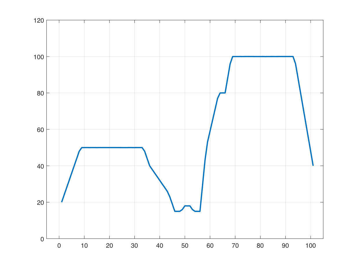
The curve I've been experimenting with is relatively smooth, with plateaus that are completely flat. Unfortunately, the imregionalmax is significantly less useful when the input is even a little noisy. That's because noise introduces small local maxima in many places, and imregionalmax picks up even the tiniest local maxima. Let's try it. If I add a very small amount of noise, you can't even see it in the plot:
rng(17)
yn = y + (0.01 * randn(size(y)));
clf
plot(x,yn)
axis([-5 105 0 120])
grid on
But now the output of imregionalmax looks completely different.
reg_max_mask_n = imregionalmax(yn);
plot(x,yn)
hold on
plot(x(reg_max_mask_n),yn(reg_max_mask_n),"*")
hold off
axis([-5 105 0 120])
grid on
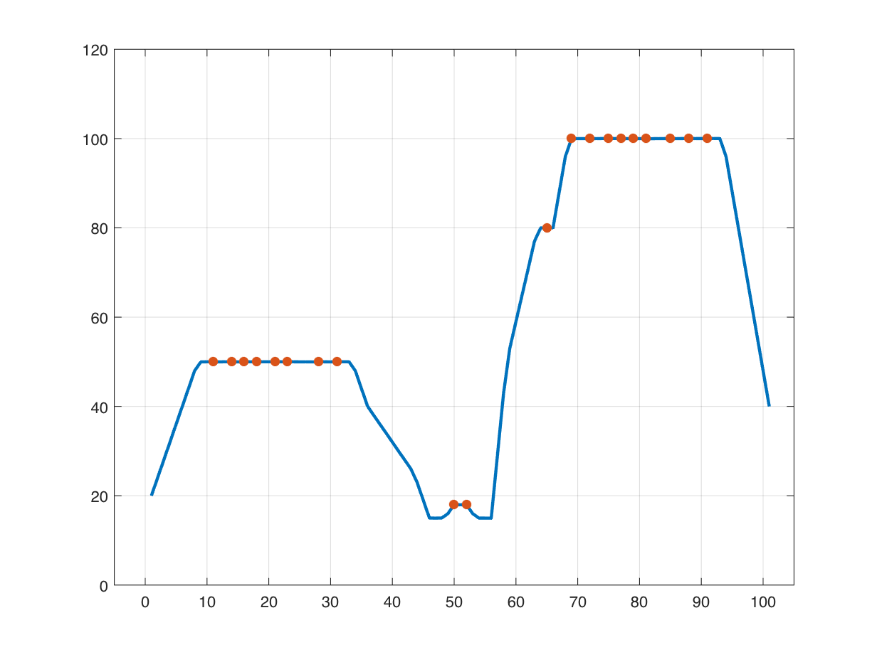
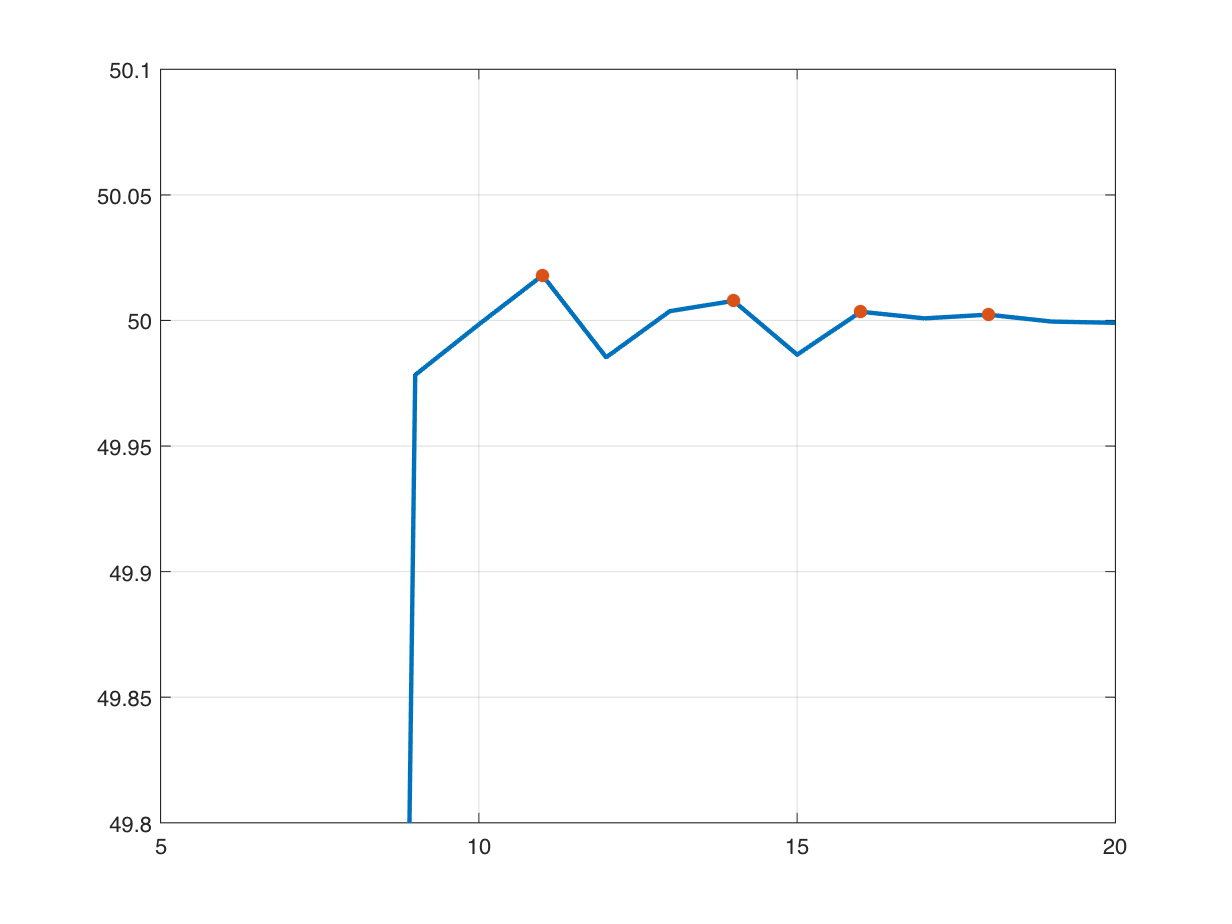
Now, only a scattering of samples on the broad plateaus are identified as regional maxima, and a sample on the small "shoulder" plateau is marked as a regional maximum where it wasn't before. We have to zoom in pretty far to see why this is happening.
axis([5 20 49.8 50.1])
axis([62 67 79.9 80.2])
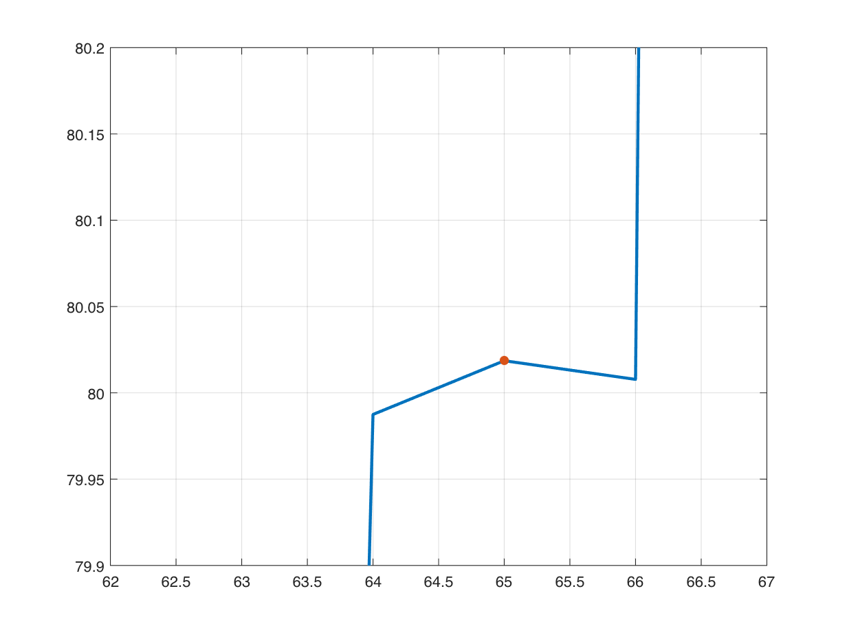
You can see that the added noise is introducing tiny local maxima in various places, and that is throwing imregionalmax off the scent from what we'd like for it to do.
imhmax
And here's where the function imhmax comes into play. It computes something called the h-maxima transform. This operation essentially suppresses any local maxima that are less than a certain height (h) above their immediate surroundings. Let's say, for example, that we are only interested in local or regional maxima that have a height of more than 5 units above their immediate surroundings. We accomplish this by calling imhmax like this:
yn_h = imhmax(yn,5);
plot(x,yn)
hold on
plot(x,yn_h)
hold off
axis([-5 105 0 120])
grid on
legend(["original" "h-maxima transform"])
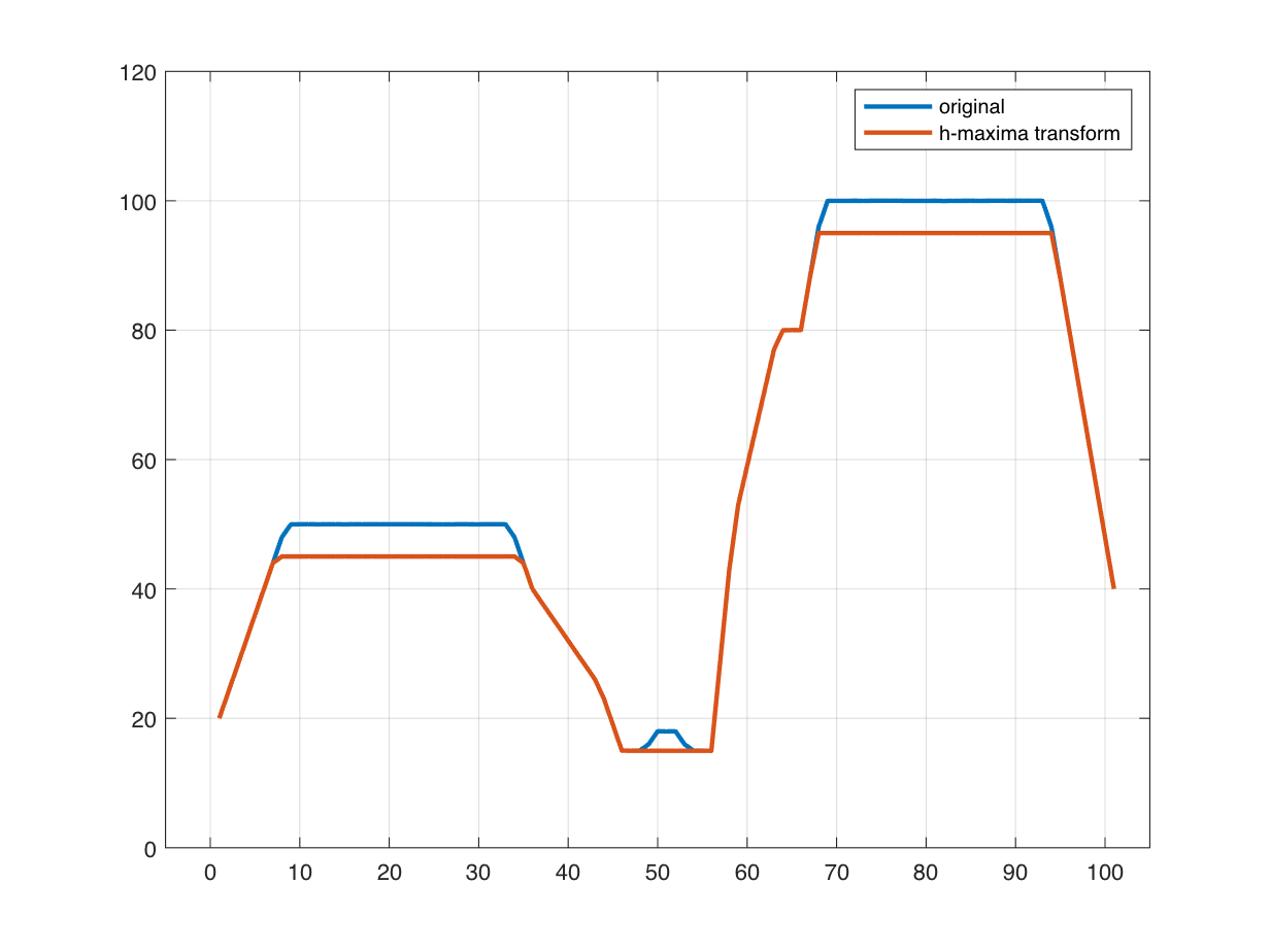
In the output of imhmax, the broad peaks have been flattened out, and the small peak in the middle, which has a height of only 3 above its surroundings, has been flattened out and eliminated. Now let's try imregionalmax again.
reg_max_mask_n_h = imregionalmax(yn_h);
plot(x,yn)
hold on
plot(x(reg_max_mask_n_h),yn(reg_max_mask_n_h),"*")
hold off
axis([-5 105 0 120])
grid on
With that computation, we have identified only the peaks that are significantly higher than what is around them, and that's often what we are interested in. Notice that the h-maxima transform spreads out the peak a bit, and so the result shown above is picking out a bit of the "shoulders" to the left and right of each broad plateau. We could do some post-processing to correct that, if necessary.
There is another function, imextendedmax, that simply combines the h-maxima transform and regional maxima steps into a single function. If you're interested in minima instead, then you can use the upside-down versions of these functions: imhmin, imregionalmin, and imextendedmin.
If you have found interesting uses for these functions in your own work, I'd love to hear about it, so please leave a comment.
Utility function
function y = peaksAndPlateaus
f = @(x) min(max(1-abs(x/5),0),0.5);
g1 = @(x) 100*f((x-20)/5);
g2 = @(x) 200*f((x-80)/5);
g3 = @(x) 30*f((x-50)/3);
g4 = @(x) 5*f(2*(x-50));
g5 = @(x) 30*f((x-60));
g = @(x) g1(x) + g2(x) + g3(x) + g4(x) + g5(x);
y = round(g(0:100));
end


Comments
To leave a comment, please click here to sign in to your MathWorks Account or create a new one.