
Local maxima, regional maxima, and the function imregionalmax
A recent algorithm discussion on the Image Processing Toolbox development team reminded me of something I originally wanted to do a long time ago: explain imregionalmax and some related operations. (I guess I got sidetracked.)
For this explanation, I'll use the following sample image:
P = sampleImage;
imshow(P)

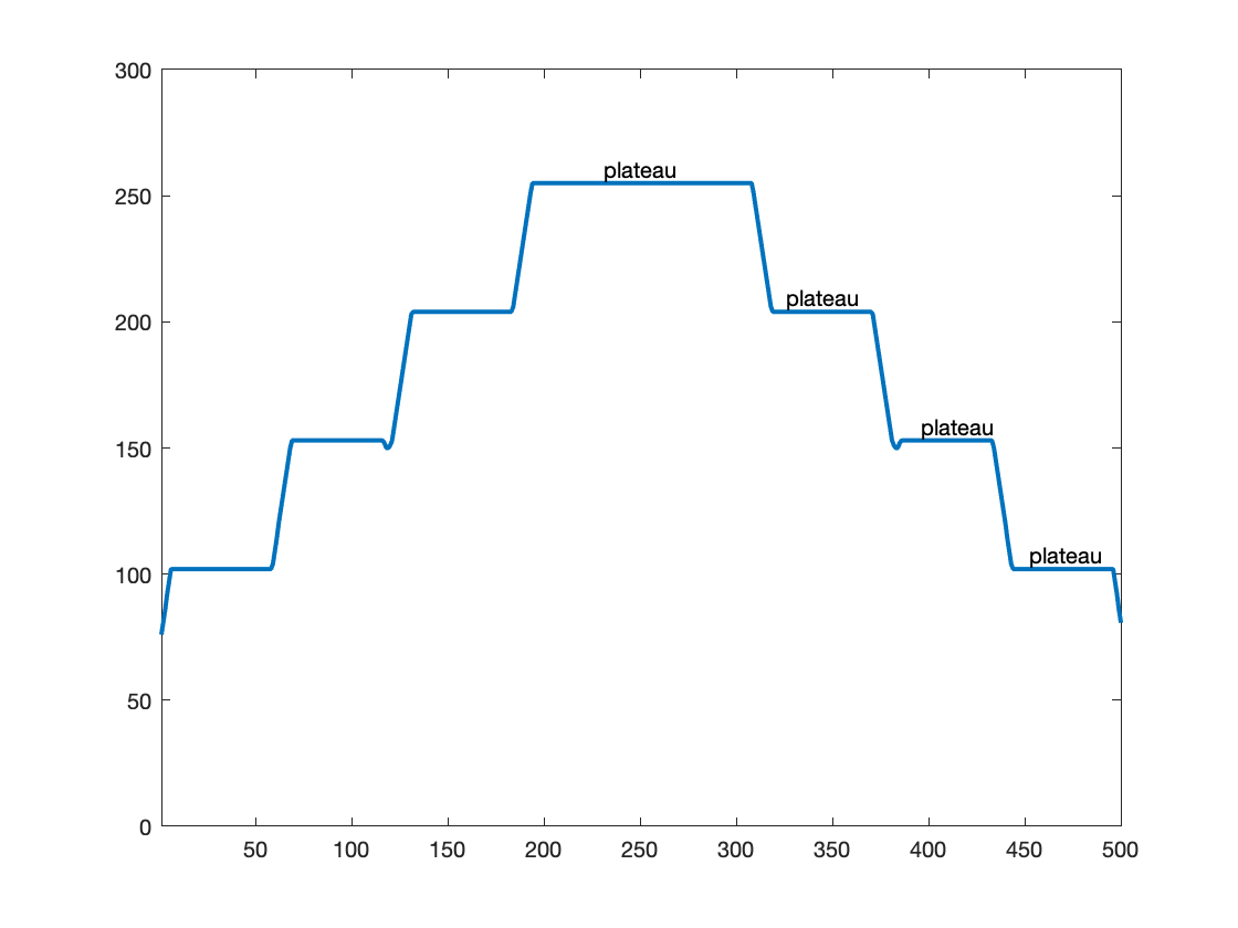
Note that this image has a number of constant-valued rings. One might call these regions "plateaus." Here is a cross-section of the pixel values:
p256 = P(256,:);
plot(p256)
axis([1 500 0 300])
text(250,255,"plateau",HorizontalAlignment = "center", ...
VerticalAlignment = "bottom")
text(345,204,"plateau",HorizontalAlignment = "center", ...
VerticalAlignment = "bottom")
text(415,153,"plateau",HorizontalAlignment = "center", ...
VerticalAlignment = "bottom")
text(471,102,"plateau",HorizontalAlignment = "center", ...
VerticalAlignment = "bottom")
Local maxima
In image processing, the usual definition of a local maximum is that a pixel is considered to be a local maximum if and only if it is greater than or equal to all of its immediate neighbors.
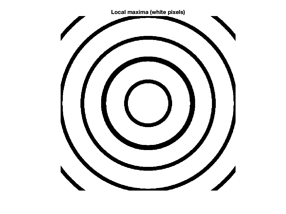
There is a convenient and efficient way to find all the local maxima pixels by using image dilation. If a pixel is unchanged following dilation, then that pixel is a local maximum.
Pd = imdilate(P,ones(3,3));
local_maxima = (P == Pd);
imshow(local_maxima)
title("Local maxima (white pixels)")
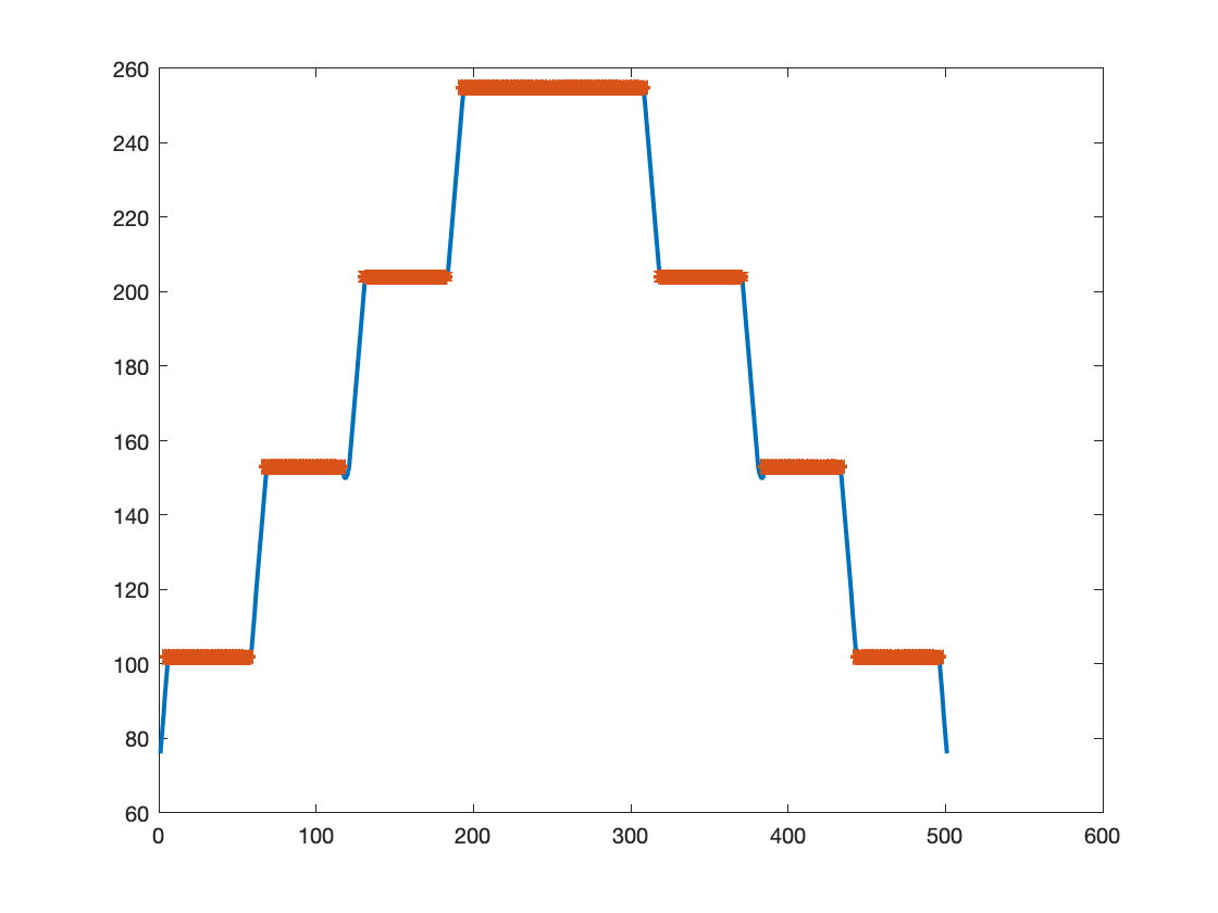
Here is a look at the local maxima along our cross section:
plot(p256)
local_maxima_256 = local_maxima(256,:);
k = find(local_maxima_256);
hold on
plot(k,p256(k),"*")
hold off
Regional maxima
Let's take a closer look at some of those plateaus and see how they differ in an important way. First, here's a closeup of the cross section of the central disk plateau:
plot(p256)
xlim([175 325])
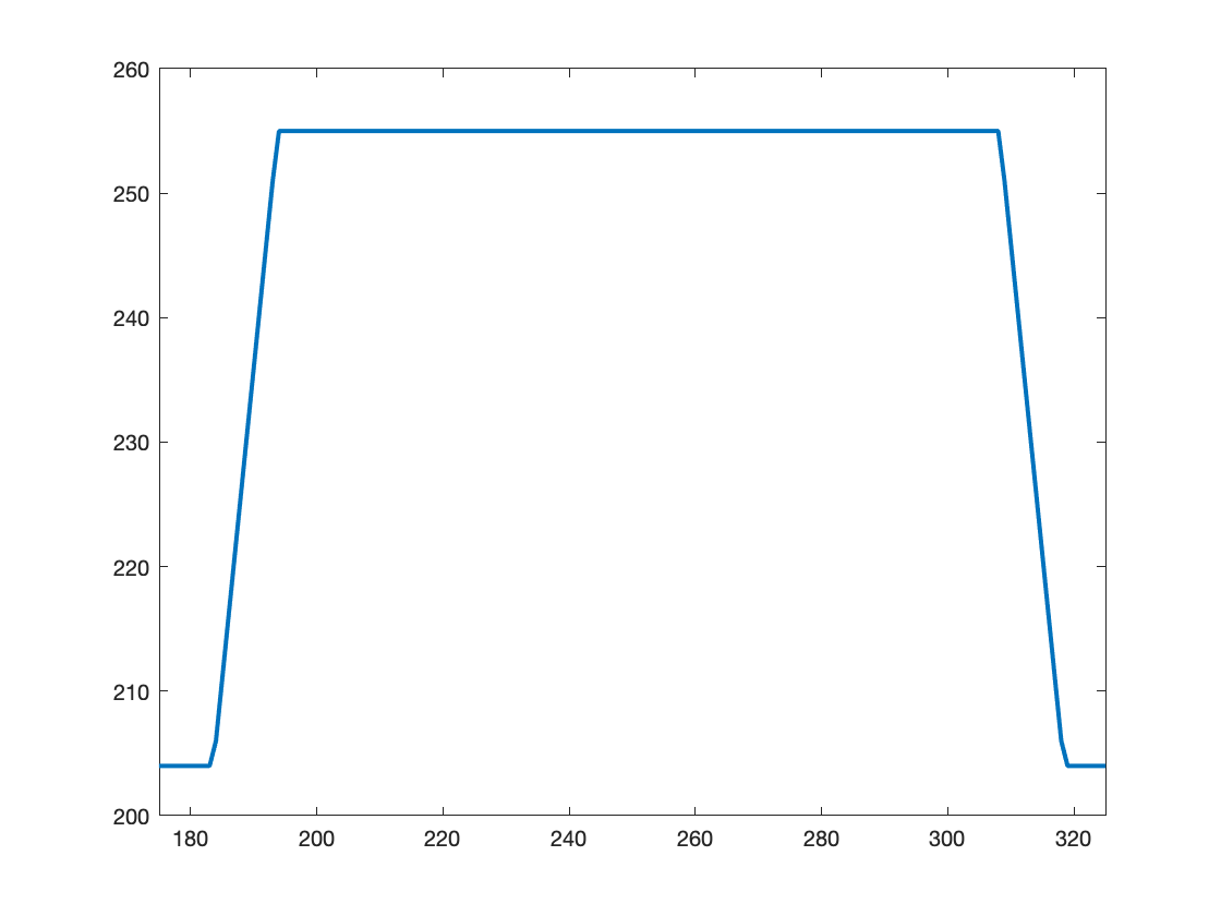
If you imagine yourself standing in the middle of that plateau, you'll realize that there's no way to move off the plateau without going downhill.
Next, let's zoom on the cross section of the first ring surrounding the central disk:
plot(p256)
xlim([315 375])
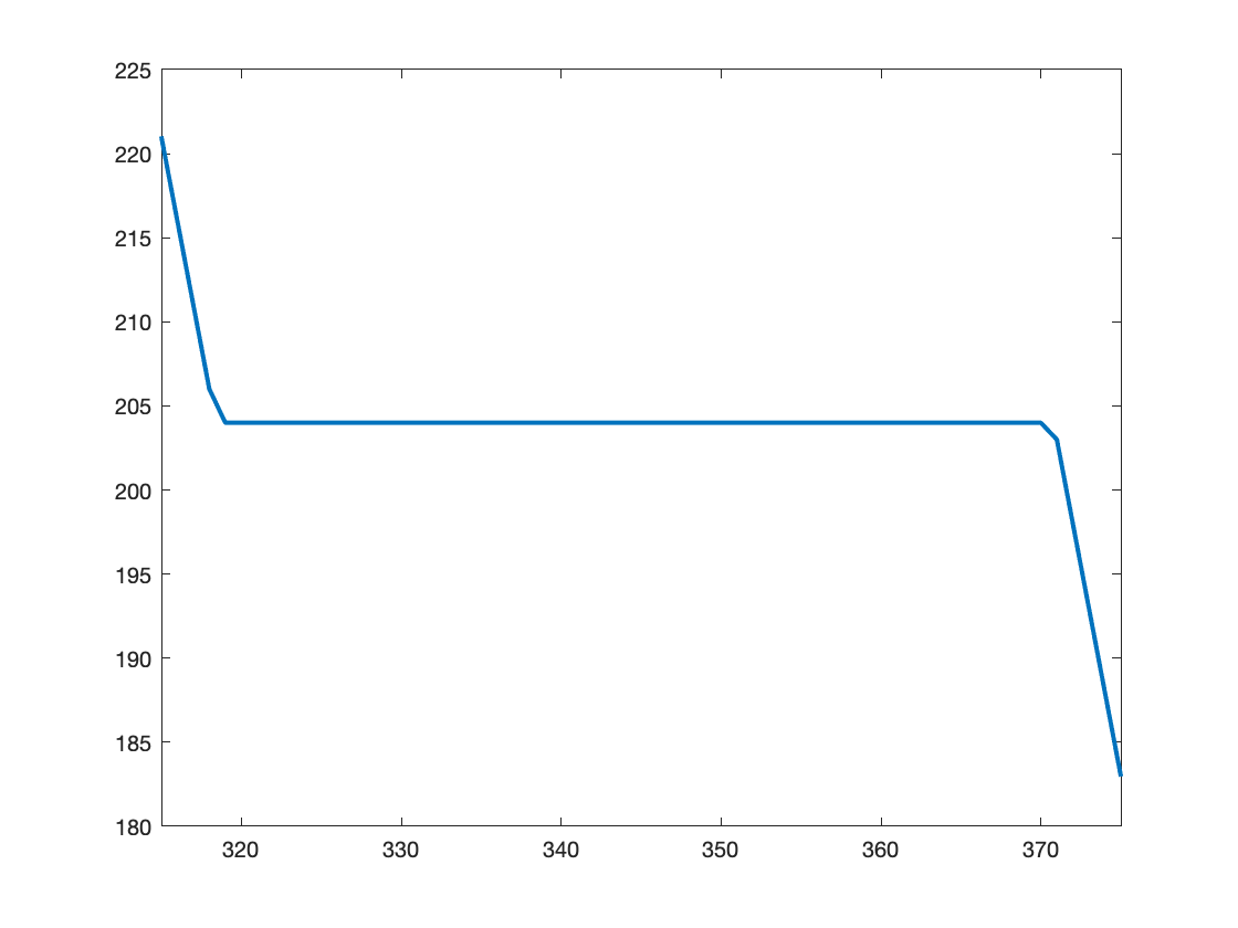
If you're standing in the middle of this plateau, then you can move off the plateau by going either down or up, depending on which direction you move in.
Now let's zoom in on the next ring:
plot(p256)
xlim([375 440])
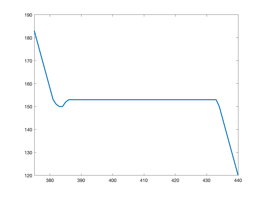
Do you see that little dip on the left side of the plateau? That means that you can't leave the plateau without going downhill. The larger trend toward the left is definitely higher, but first you have to go down that dip.
Considering these different plateaus leads to our formal definition of a concept called regional maximum: a connected component of pixels with a constant value h (that's the plateau), where every pixel that is neighbor to that connected component has a value that is lower than h (that is, every neighboring pixel of the plateau is downhill from it).
And that is what imregionalmax computes.
Function imregionalmax
The function imregionalmax takes a grayscale image and returns all of the regional maxima pixels in the form of a binary mask. Here's what the function produces from our sample image. I'll show it side-by-side with the local maxima mask from above for easy comparison.
regional_maxima = imregionalmax(P);
tiledlayout(1,2)
nexttile
imshow(local_maxima)
title("Local maxima")
nexttile
imshow(regional_maxima)
title("Regional maxima")
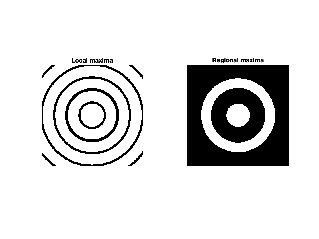
You can see that only the central disk and the second ring (from the center) have been marked as regional maxima.
Generally, if you are looking for peaks in an image, and if your image can have plateaus in it, then you are probably better off looking for regional maxima rather than local maxima.
However, the location of regional maxima can be very sensitive to even very small, noisy variations in pixel values. So, I'm going to write another post soon about the h-maxima transform and the functions imhmax and imextendedmax.
Stay tuned!
Utility functions
function out = sampleImage
x = linspace(-100,100,501);
r = hypot(x,x');
out = zeros(size(r));
rings = 25:25:125;
% for k = 1:length(rings)
% out = out + tanh((rings(k) - abs(r))./2);
% end
% out = out - 0.15*exp(-((r-54)/3).^2);
for k = 1:length(rings)
out = out + profile((rings(k) - r)/2);
end
out = out - 0.15*triangle(r-53);
out = im2uint8(mat2gray(out));
end
function y = profile(x)
y = min(abs(x),1) .* sign(x);
end
function y = triangle(x)
y = max(1-abs(x),0);
end


Comments
To leave a comment, please click here to sign in to your MathWorks Account or create a new one.