
Differential Equations Modeling with MATLAB – SCUDEM
Joining us today is Wesley Hamilton, who is a STEM Outreach Engineer here at MathWorks. Wesley will talk about SIMIODE’s SCUDEM competition. Wesley, over to you…
Overview
This blog post has three goals:
- Introduce SIMIODE’s SCUDEM competition, which MathWorks now supports,
- Show how one might start developing a model to address a real world (SCUDEM) problem, and
- Showcase the ODE solving functionality provided by MATLAB.
We’ll be showcasing how a new team to SCUDEM, and math modeling, might get started developing a solution to a problem. As such the model won’t be particularly refined, but the modeling process employed can (and should) be replicated as a better practice when competing.
SIMIODE and SCUDEM
The Systemic Initiative for Modeling Investigations and Opportunities with Differential Equations (SIMIODE) is an organization that, as described on their website, “is a Community of Practice focused on a modeling first method of teaching differential equations”. Since 2017, SIMIODE has organized the SIMIODE Challenge Using Differential Equations Modeling (SCUDEM). This annual competition has teams pick one of three problems, and develop a differential equation model to answer their chosen problem. This year SCUDEM will run from October 20 to November 30, in which time teams will develop their models and prepare a short youtube video describing their work. The SCUDEM website has more information on taking part, including registration information and problems and results from previous years.
This year, MathWorks is excited to provide direct support for SCUDEM by way of licenses and preparatory materials. Read on for some of these new preparatory materials.
The problem
For this blog post, we’re going to tackle the 2022 SCUDEM problem A, which ask teams to develop a model that describes ISS astronauts’ stress when completing tasks and helping/getting helped by ISS visitors. Take a minute to read through the problem statement in its entirety by going to https://qubeshub.org/community/groups/scudem/wiki/SCUDEMVII2022, and then click on “Problem Statements” underneath “Official Challenge Problems for SCUDEM VII 2022”. A PDF with all three of the 2022 problem statements will be downloaded.
Before setting up a model, we need to have a solid grasp of the actual problem we’re being asked to address. Here, let’s walk through the problem statement paragraph by paragraph and pick out key pieces that will help us specify what exactly we’re building a model for.
A group of individuals recently purchased a flight to go to the International Space Station [1]. Each of them had to complete a rigorous training regime and demonstrate that they were capable of handling the physical and mental demands of space travel. When they arrived, they were expected to provide help and assistance to the astronauts who were at the station and the new crew members had a large number of tasks and experiments to complete.
In the model we develop, we’re going to specify two different groups of people that may behave (and be modeled) differently. Since the ISS has a smaller number of crew, we have two options to explore:
- follow a more agent-based model approach, where we keep track of individual astronauts and visitors, or
- treat the astronauts and visitors as single entities, so that we’re modeling e.g. the collective stress of the astronauts and not individuals’ stress.
Either approach can work, and both approaches may not be difficult to implement in MATLAB. Let’s read on to see what other information might inform which of these options we’ll pick.
The hectic schedule nearly overwhelmed the newly arrived guests, and the extra attention they required added to the stress felt by the existing crew. What can be done to ease this burden, yet result in a more efficient use of time for a flight crew? Before answering this question, a way to model the stress and capabilities of a flight crew must be created.
A key piece of information is that “stress” and “capabilities” are explicitly mentioned. At this point, these may be the two quantities we build a model around for each group or each astronaut/visitor. Moreover, the specific mention that the visitors added to the stress of the astronauts is important – when we test our model, we may want to run a simulation without visitors to confirm that the stress of the astronauts is stable (in some capacity), since the provided information suggests that the visitors potentially threw things out of stability.
Develop a mathematical model of the stress and capabilities of a group of people. Assume that there is an existing group of people in place at the destination who are already under a great deal of pressure to complete their assigned tasks. The model should include the addition of a second group of capable people who arrive after undergoing the stress of a space launch and do not have prior exposure to the new environment. Given the expected stress levels over time what is the impact on the whole group?
This paragraph has the main task: Develop a mathematical model of the stress and capabilities of a group of people. As above, we’re still looking at focusing on stress and capability as the two numeric quantities to use, and the specific mention of a group of people suggests it’s not out-of-line to treat all astronauts as a single entity (the group of astronatus), and same with the visitors. Otherwise, we’re being asked to say something about stress levels over time – if in the end we don’t want to keep track of both stress and capabilities, then we should definitely keep stress as the main quantitative object we work with.
Your model should be able to take a schedule for the whole group and then predict the impact on the group of people. You should identify what happens under different scenarios including the expectation of an immediate high level of productivity, a short period of rest followed by a sharp rise in a high level of productivity, and then a gradual increase from low to high levels of productivity. Which scenario results in the lowest stress and highest net productivity? Also, what should ground observers expect from small deviations from a given schedule?
Here we’re given a few more specific requirements to include:
- incorporate a schedule for the astronauts and visitors,
- incorporate different levels of productivity for all onboard,
- incorporate (small) deviations in the schedule.
All of this should be incorporated to say something about the long-term stress of everyone onboard.
So to summarize (some of) what we’ve picked out of the problem statement:
- model the stress and capabilities for astronauts and visitors, and
- incorporate a schedule with varying amounts of productivity each day.
In the next section, we’ll identify how we want to quantify everything before incorporating our initial model in MATLAB.
An initial model – plan
Models can be as complex or as simple as one desires. Here, we’ll start with developing a simple model to showcase a viable approach, which will hopefully give us some preliminary results and pave the way to a more complex, and descriptive of the situation, model.
To start, let’s just model the stress of the astronauts and visitors and incorporate capabilities through the model parameters; later on we may revisit this decision and look more closely into how capabilities and stress interact. Thus, our functions of interest will be
- $ s_a $ for the stress of astronauts, and
- $ s_v $ for the stress of the visitors,
and our system of differential equations will look like
$ \frac{ds_a}{dt} = … $
$ \frac{ds_v}{dt} = … $
There are a few ways we might model the change in stress, and since we’re not trained specialists in the psychology of stress, we’ll rely heavily on assumptions to set up our model. Let’s start by developing the model for an astronaut’s stress, and then look at how a visitor’s stress is incorporated.
We’ll assume that the increase in stress is proportional to the amount of work being done and the amount of stress already accumulated, and stress decreases while at rest at a rate proportional to their current stress level: for this we’ll need
- a constant of proportionality for stress accumulation $ \alpha_a $,
- a constant of proportionality for stress decumulation $ \beta_a $, and
- a function detailing the amount of work an astronaut is doing $ W(t) $.
As the astronaut is working ($ W(t)>0 $), their total stress should increase. When the astronaut is at rest ($ W(t)=0 $), their total stress should decrease. For our initial approach let’s assume that astronauts work at a constant rate of $ W(t)=1 $ when on-duty. With this framework we can write
$ \frac{d s_a}{dt} = \alpha_a W(t) s_a(t) – \beta_a s_a(t) (1 – W(t)) $.
Since there was nothing specific in this framework to astronauts, we’ll assume visitor stress follows the same model (with their own constants of proportionality:
$ \frac{d s_v}{dt} = \alpha_v W(t) s_v(t) – \beta_v s_v(t) (1 – W(t)) $
In future versions of this model, we may modify the work function to be different for astronauts and visitors, but for now we’ll stick with this approach.
Next, we need to discuss the interaction of stress between astronauts and the visitors. An initial assumption we’ll make is that an astronaut’s stress accumulation is also proportional to the stress of the visitors, and vise versa, so our equations become
$ \frac{d s_a}{dt} = \alpha_a W(t) s_a(t)s_v(t) – \beta_a s_a(t) (1 – W(t)) $,
$ \frac{d s_v}{dt} = \alpha_v W(t) s_a(t)s_v(t) – \beta_v s_v(t) (1 – W(t)) $.
Once we run simulations we can start specifying the constants that make sense for our model, but we do need to specify ahead of the simulation, based on astronauts’ actual schedules. For this, we can do some research; this article suggests astronauts work from 6 am to 9.30 pm, with three meals and 2.5 hours of exercise. Without a specific schedule to copy, we’ll make the following assumption for the astronauts’ and visitors’ schedule:
- astronauts wake up at 6 am but spend 60 minutes for breakfast/working out/taking a break, so work starts at 7 am;
- astronauts work for 4 hours until 11 am, and then take 90 minutes for lunch/working out/taking a break, so work resumes at 12.30 pm;
- astronauts work for 5 hours until 5.30 pm, before taking another 90 minutes for dinner/working out/taking a break, until work resumes at 7 pm;
- astronauts work for 2 hours until 9 pm before taking a final 30 minute break, before going to bed at 9.30 pm.
This rough schedule include the 2.5 hours of exercise, as well as another 2 hours for assorted meals and breaks.
From the perspective of our work function $ W(t) $, using a 24-hour clock, this means that
$ W(t) = 1 $ for $ 7\leq t\leq 11 $, $ 12.5\leq t\leq 17.5 $, $ 19\leq t\leq 21.5 $, and
$ W(t) = 0 $ otherwise.
All calculations should be done modulo 24 since we want to track stress over a few days.
Here it’s worth reiterating that this model is quite basic, and that’s okay! We’re trying to establish a baseline model before we start refining our assumptions and extending our model to more accurately address what the problem statement is actually asking for.
Next, let’s implement our model in MATLAB!
An initial model – implementation in MATLAB
Let’s start by implementing just the model for astronauts’ stress levels. Our goal is to establish a baseline for our constants of proportionality, before we incorporate the visitors. In particular, our expectation is that astronauts’ stress levels should be stable over a few days, so we need to specify constants that respect this expectation.
Since we want to simulate stress over time, we’ll be using MATLAB, and in particular MATLAB’s ODE functionality. With the release of MATLAB 2023b there is some slick functionality for setting up and solving ODEs – our approach follows this new functionality as described in this recent blog post.
First, let’s encode the work function. Because of the nature of LiveScripts the actual function is included at the end of this post, but the monospace that follows is a direct copy of that function:
function w = W(t)
normT = mod(floor(t),24) + (t – floor(t));
if (normT >= 7) && (normT <= 11)
w = 1;
elseif (normT >= 12.5) && (normT <= 17.5)
w = 1;
elseif (normT >= 19) && (normT <= 21)
w = 1;
else
w = 0;
end
end
In particular, note that since we’re running our model a few days into the future, we need to convert from the time that the mission started to a local 24-hour clock.
Next, let’s incorporate the constants of proportionality using sliders; the intention here is to experiment to identify reasonable values for the astronauts and their stress levels:
alphaA = 0.3;
betaA = 2;
initValA = 0.3;
Finally, let’s write down the function $ \frac{ds_a}{dt} $ :
dsa = @(t,y) alphaA*y*W(t) – betaA*y*(1-W(t));
With these pieces in place, we can now solve the ODE and see what the astronauts’ stress levels over time is:
initF = ode(ODEFcn=dsa,InitialTime=7,InitialValue=initValA); % Set up the problem by creating an ode object
sol = solve(initF,7,100); % Solve it over the interval [0,10]
plot(sol.Time,sol.Solution,“-o”)

Next, let’s incorporate the addition of the visitors. To do this, we need the new set of constants of proportionality, as well as a new function describing the differential equation that will look similar to what we had before:
alphaV = 0.9;
betaV = 1.5;
initValV = 0.5;
Here we’re assuming that the visitors get stressed more easily ($ \alpha_v > \alpha_a $), and don’t destress as easily ($ \beta_v < \beta_a $). Otherwise, our function for the system of equations should now be a vector (the first coordinate is the astronauts’ stress, and the second coordinate is the visitors’ stress):
ds = @(t,y) [alphaA*y(1)*y(2)*W(t) – betaA*y(1)*(1-W(t)); alphaV*y(1)*y(2)*W(t) – betaV*y(2)*(1-W(t))];
F = ode(ODEFcn=ds,InitialTime=7,InitialValue=[initValA;initValV]); % Set up the problem by creating an ode object
sol = solve(F,7,100); % Solve it over the interval [0,10]
plot(sol.Time,sol.Solution,“-o”)

As above, the blue curve is the stress of astronauts, while the orange curve is the stress of the visitors.
Try playing around with the parameters, and you’ll see that it’s easy for, after the addition of visitors, stress levels to blow out of control. With that said, we were able to find a range of parameters that suggest, at least with these assumptions, the astronauts and visitors are able to eventually find harmony in their working conditions.
Next steps
To reiterate: this is a very, very basic, initial model for human stress. While we have some preliminary results from this model that are interpretable, there are several modifications we can do to make the model even more descriptive and realistic, including, but not limited to:
- modifying the working function $ W(t)% $ to incorporate the working conditions specified in the problem statement,
- (possibly) modifying the stress interactions for individuals, and not the cumulative group,
- revisiting the initial model for the changes in stress, possibly adding crew capabilities for performing work as another function,
- etc.
Interested in more? Check out some of our other preparatory materials for MATLAB and math modeling listed on the SCUDEM website, as well as other MathWorks blogs for more ideas, tips, and tricks on how to effectively use MATLAB.
Functions
function w = W(t)
normT = mod(floor(t),24) + (t – floor(t));
if (normT >= 7) && (normT <= 11)
w = 1;
elseif (normT >= 12.5) && (normT <= 17.5)
w = 1;
elseif (normT >= 19) && (normT <= 21.5)
w = 1;
else
w = 0;
end
end
- Category:
- Math Modeling,
- MATLAB


Comments
To leave a comment, please click here to sign in to your MathWorks Account or create a new one.