Using Lidar for 3D Object Detection

Posted by Tanya Kuruvilla, June 1, 2026

17 views (last 30 days) | 0 Likes | 0 comment

Today, we’re going through each step of creating a 3D object detector using Lidar data. We’ll start with an introduction to 3D point clouds and how to process them, then we’ll label point clouds for deep learning, train an 3D object detector, and wrap up by discussing a few options for deploying the detector to your projects or hardware.

The complete dataset, code, and videos we’ll be discussing in this blog can be found at this GitHub Repository.

Understanding and Processing Point Clouds
Labeling Point Clouds for Deep Learning
Training a 3D Object Detector with Deep Learning
Deploying a 3D Object Detector

1. Understanding and Processing Point Clouds

The dataset used in this example can be found in this ‘parkingLot’ folder and will need to be downloaded in order to follow along. A video explanation of this topic can be found here.

Understanding Point Clouds

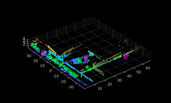
Lidar sensors record spatial data and store it as a point cloud, or a collection of points that represent the world around the sensor. In a 3D point cloud, these points are stored as x,y,z coordnates and can be visualized, so if your environment looks like this:

your point cloud might look like this:

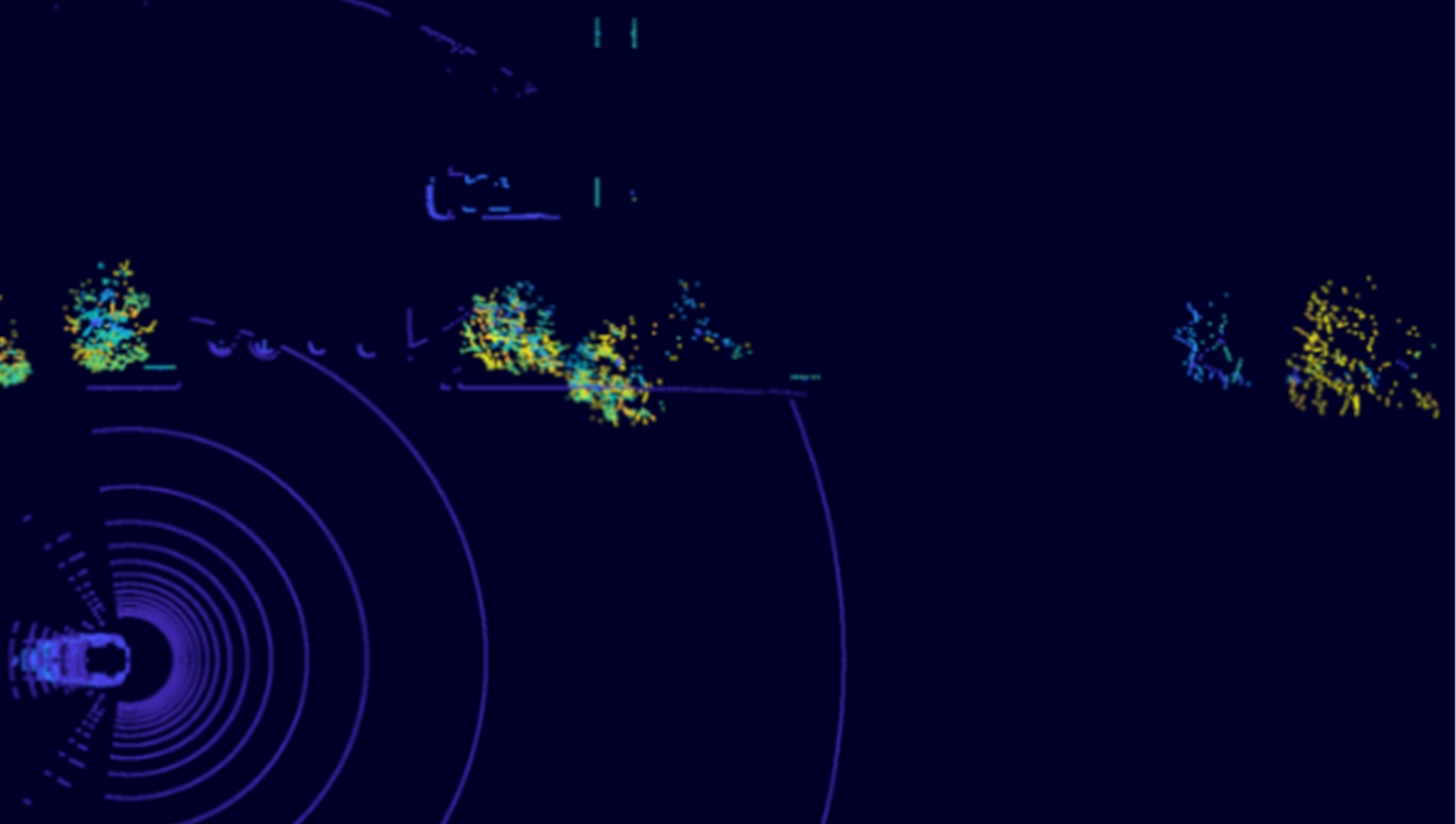
This is a way of numerically representing the world around us in 3 dimensions, which is helpful for developing algorithms that rely on things like distance from a robot or size of an object.

Processing Point Clouds

Processing point clouds before using them for deep learning can often lead to better results. The Lidar Viewer App lets you import, view, and process point clouds interactively, and is demonstrated in this video.

You can also process point clouds programmatically. Load in a point cloud from our dataset using the pcread function:

singlePtCld = pcread(‘./parkingLot/frame_0001.pcd’);

pcshow(singlePtCld)

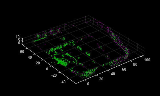
Denoising

Point clouds can have “noise”, or data points that are outliers to what you’d expect to see in your point cloud. Use the pcdenoise function to remove or reduce these. The purple points in the figure below represent points that were removed.

ptCloudDenoise = pcdenoise(singlePtCld);

figure

pcshowpair(singlePtCld, ptCloudDenoise)

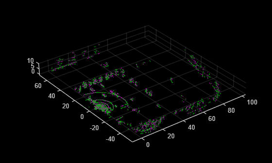
Downsampling

Depending on your LiDAR and the environment you collected data in, you may have a lot of data points, which can lead to slower computaton. Use the pcdownsample function to make your point cloud less dense through downsampling. Use pcshowpair to view which data points were removed (purple) and which stayed (green).

ptCloudDownSampled = pcdownsample(ptCloudDenoise,‘random’,0.60);

pcshowpair(ptCloudDenoise, ptCloudDownSampled)

Check out this documentation page to see further options for processing lidar data.

It can be helpful to test out different preprocessing methods on a single point cloud to see how it affects your data. Once you have a combination of steps and settings that you’re happy with, you can apply it to the whole dataset. This is easy to do with the Lidar Viewer app, which exports the processed dataset to a folder called parkingLot_Edit by default.

2. Labeling Point Clouds for Deep Learning

Once the data is processed, you can label the objects in the point clouds. First, split the data into a train and test dataset, which helps for the deep learning step.

pcd_files = dir(“./parkingLot_Edit/*.pcd”);

test_data = pcd_files(1:366);

train_data = pcd_files(367:807); 

if ~exist(“./parkingLotTrain”, ‘dir’)

 mkdir(“./parkingLotTrain”);

end

if ~exist(“./parkingLotTest”, ‘dir’)

 mkdir(“./parkingLotTest”);

end

for i=1:length(train_data)

 fileName = fullfile(train_data(i).folder, train_data(i).name);

 copyfile(fileName, “./parkingLotTrain”);

end

for i=1:length(test_data)

 fileName = fullfile(test_data(i).folder, test_data(i).name);

 copyfile(fileName, “./parkingLotTest”);

end

For this example, we label cars, cones, and barrels using the Lidar Labeler app. You can start a new labeling session by running the ‘lidarLabeler’ command below

lidarLabeler

or by selecting the Lidar Labeler app from the ‘APPS’ tab.

Watch this video to see how we label the dataset and save the labels to a variable called gTruth:

3. Training a 3D Object Detector with Deep Learning

With a labeled dataset, it’s time to train your object detector! A video explanation of this topic can be found here.

Import Labeled Data

Create datastores to access the data and associate labels with their corresponding point clouds.

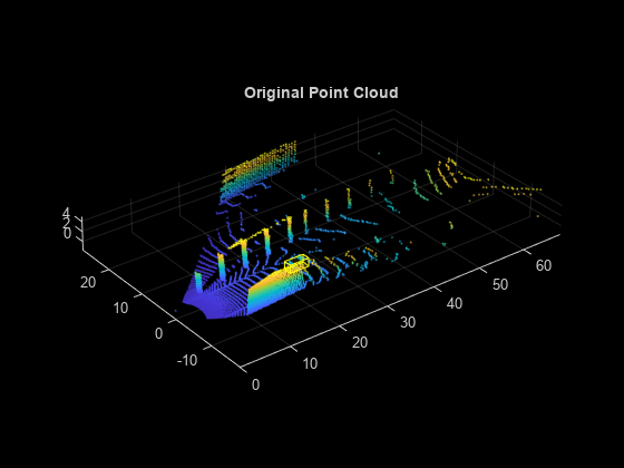
[pcds,bxds] = lidarObjectDetectorTrainingData(gTruth, “SamplingFactor”,1);

dsTrain = combine(pcds, bxds);

preview(dsTrain)

ans = 1×3 cell 

1
2
3

1
1×1 pointCloud
4×9 double
4×1 categorical

	1	2	3
1	1×1 pointCloud	4×9 double	4×1 categorical

When you read from the datastore dsTrain, it returns a point cloud, bounding boxes of each object in the point cloud, and the labels for each bounding box.

Augment the Data

Augmentation is a great way to make your dataset, and therefore your object detector, more robust. Use the sampleLidarData function to collect point cloud samples from each of the classes present in the data.

classNames = [“car”, “barrel”, “cone”]; 

sampleLocation = fullfile(pwd, “parkingLotSampled”);

[ldsSampled,bdsSampled] = sampleLidarData(dsTrain,classNames,…

 WriteLocation=sampleLocation,Verbose=false);

dsSampled = combine(ldsSampled,bdsSampled);

Then, apply the ‘pcBboxOversample’ function to insert these samples into each point cloud, ensuring that each point cloud will have at least 3 of each object. The images below are an example of what this process looks like.

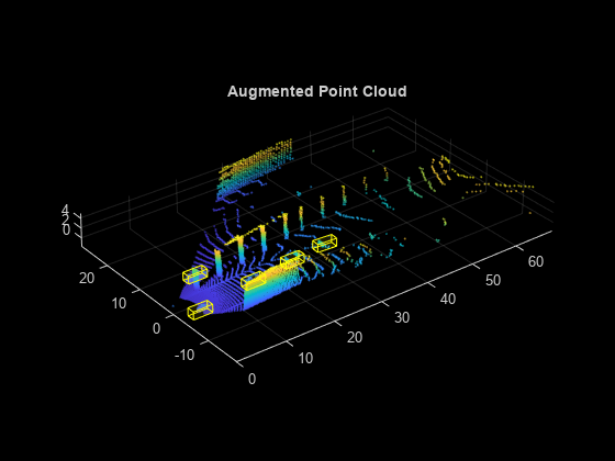
totalObjects = 3;

dsOversampled = transform(dsTrain,…

 @(x)pcBboxOversample(x,dsSampled,classNames,totalObjects));

Configure Object Detector

Specify the point cloud range, class names, and anchor boxes that you’ll use to train the detector.

anchorBoxes = calculateAnchorsPointPillars(gTruth.LabelData);

xMin = 0;

xMax = 69.12;

yMin = -39.68; 

yMax = 39.68;

zMin = -0.5157;

zMax = 5;

pcRange = [xMin, xMax, yMin, yMax, zMin, zMax];

pretrainedDetector = load(“pretrainedPointPillarsDetector.mat”,“detector”);

oldDetector = pretrainedDetector.detector;

detector = pointPillarsObjectDetector(oldDetector.Network,pcRange,classNames,anchorBoxes);

Use the trainingOptions function to specify how the model will be trained. Choosing training options is an iterative process, so try adjusting some of these options and see how it affects the performance of your detector.

options = trainingOptions(‘adam’,…

 ‘MaxEpochs’,60,…

 ‘MiniBatchSize’,3,…

 ‘GradientDecayFactor’,0.9,…

 ‘SquaredGradientDecayFactor’,0.999,…

 ‘LearnRateSchedule’,“piecewise”,…

 ‘InitialLearnRate’,0.0002,…

 ‘LearnRateDropPeriod’,15,… 

 ‘LearnRateDropFactor’,0.8,…

 ‘BatchNormalizationStatistics’,‘moving’,…

 ‘ResetInputNormalization’,false);

Train Object Detector

Use the trainPointPillarsObjectDetector function to train your network!

[detector,info] = trainPointPillarsObjectDetector(dsOversampled,detector,options);

Test Object Detector

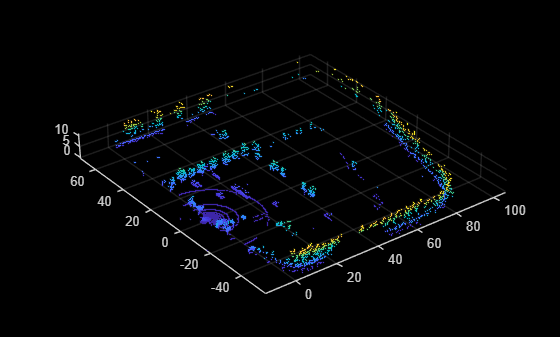
Now that you have a trained detector, test it on a frame from the test set:

player = pcplayer([xMin xMax],[yMin yMax],[zMin zMax]);

testframe = pcread(‘./parkingLotTest/frame_0014.pcd’);

view(player,testframe);

ax = player.Axes;

[bboxes,scores,labels] = detect(detector,testframe,“Threshold”,0.4);

showShape(“cuboid”,bboxes,Color=“green”,Parent=ax,Opacity=0.3,LineWidth=1);

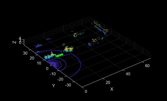
By showing the detected objects, we can see that the detector is successfully detecting the row of barrels!

Once you have a 3d object detector that you’re happy with, save it to a .MAT file for later use.

save detector detector

4. Deploying a 3D Object Detector

You will need to do some setup before you can deploy a neural network. Watch this video to learn more about the setup steps and for an explanation of the following options.

Generate a static library
Generate an executable ROS2 node

Option 1: Generating a Static Library

To get started, create an inference function called pillarPredict that loads the trained network, makes a prediction, and returns the detection results.

function [bboxes, scores, labels] = pillarPredict(pcloud_3d, intensities)

%#codegen

 persistent mynet

 if isempty(mynet)

 mynet = coder.loadDeepLearningNetwork(‘detector.mat’);

end

 %Converting to pointCloud so the model can detect objects. pointCloud

 %function can be used in code generation

 pcloud = pointCloud(pcloud_3d, Intensity=intensities);

 [bboxes,scores,labels] = detect(mynet,pcloud,‘Threshold’,0.5);

end

Then, create an entry point script. This helps in defining the input and output variable types and shapes.

% Load a test data point and convert it from point cloud to 3D array

pcloud = pcread(“..\testData\frame_0001.pcd”);

pcloud_3d = pcloud.Location;

intensities = pcloud.Intensity;

[bboxes, scores, labels] = pillarPredict(pcloud_3d, intensities);

Now, open MATLAB Coder and set it up to generate a static library. The code generation function will be the pillarPredict function and the entry point script is the entry point function shown above.

coder

Ensure that ‘Enable code generation for deep learning’ is checked and the right library is used. This can be set under Settings -> Deep Learning as shown below.

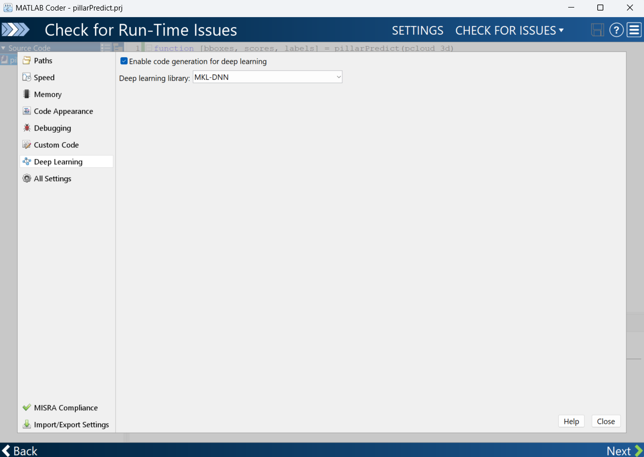
The next step is to generate code. Here, choose a static library, then click ‘Generate’ to begin code generation. The static library can then be used with your project!

ROS Node Generation

These steps show how to generate a ROS2 node that subscribes to a point cloud message and publishes the inference of the trained network. To get started, setup MATLAB Coder to generate a ROS2 node and to use the appropriate deep learning library. For this example, we’ll generate a node that can run on a Jetson Orin Nano using the CUDNN library, which uses CUDA cores to speed up inference.

% Setup the coder to generate a ROS2 node on a remote device

cfg = coder.config(“exe”);

cfg.Hardware = coder.hardware(“Robot Operating System 2 (ROS 2)”);

cfg.Hardware.DeployTo = “Remote Device”;

cfg.Hardware.BuildAction = “Build and run”;

% The Jetson board has an ARM 64 bit processor so we choose that as the device type

cfg.HardwareImplementation.ProdHWDeviceType = “ARM Compatible->ARM 64-bit (LLP64)”;

cfg.HardwareImplementation.ProdLongLongMode = true;

% The next three lines sets up the GPU coder and sets up to use CUDNN

cfg.GpuConfig = coder.GpuCodeConfig;

cfg.GpuConfig.Enabled = true;

cfg.DeepLearningConfig = coder.DeepLearningConfig(‘cudnn’);

% The last 4 lines provides information of the remote device so the coder

% can transfer the generated code and build it.

cfg.Hardware.RemoteDeviceAddress = ‘172.21.89.193’;

cfg.Hardware.ROS2Workspace = ‘/home/ubuntu/ros2_ws’;

cfg.Hardware.RemoteDeviceUsername = ‘ubuntu’;

cfg.Hardware.RemoteDevicePassword = ‘ubuntu’;

With the coder setup, you can create a MATLAB ROS2 node that can then be used to generate a CUDA ROS node. The below function lidarInfer creates a simple node that subscribes the topic “static_cloud” (which is being published by another node that reads the point cloud file) and publishes the bounding box location and object labels.

function lidarInfer()

 %#codegen

 node = ros2node(“/detector_node”);

 pclSub = ros2subscriber(node, “/static_cloud”,“sensor_msgs/PointCloud2”);

 % Create a bounding box publisher

 bboxPub = ros2publisher(node, ‘/bbox’,‘std_msgs/Float32MultiArray’);

 bboxMsg = ros2message(“std_msgs/Float32MultiArray”);

 % Create a label publisher

 labelPub = ros2publisher(node, ‘/label’, ‘std_msgs/String’);

 labelMsg = ros2message(“std_msgs/String”);

 r = ros2rate(node, 30);

 reset(r);

We set the rate to 30Hz, but this would depend on the hardware you use and the inference speed that can be achieved along with the rate at which the Lidar is publishing.

 while(1)

 [data, ~, ~] = receive(pclSub, 5);

 if ~isempty(data)

 % Using raw data to pass to the predict function since a pointcloud object cannot be passed to a code generation function

 rawData = rosReadXYZ(data);

 [bboxes, scores, labels] = pillarPredict(rawData);

 [~,idx] = max(scores);

 bboxMsg.data = zeros(6, 1, ‘single’);

 labelMsg.data = ”;

 if ~isempty(scores)

 bboxMsg.data = single(bboxes(idx,:)’);

 label_data = cellstr(labels(idx));

 labelMsg.data = label_data{1};

end

 send(bboxPub, bboxMsg);

 send(labelPub, labelMsg);

end

 waitfor(r);

end

end

The main loop shown above reads the point cloud message and then passes it to the pillarPredict function shown below, which loads the trained network and returns the inference results. The results are then passed into the bounding box and label variables before being published.

function [bboxes, scores, labels] = pillarPredict(pcloud_3d)

%#codegen

 persistent mynet

 if isempty(mynet)

 mynet = coder.loadDeepLearningNetwork(‘detector.mat’);

end

 %Converting to pointCloud so the model can detect objects. pointCloud

 %function can be used in code generation

 pcloud = pointCloud(pcloud_3d);

 [bboxes,scores,labels] = detect(mynet,pcloud,‘Threshold’,0.5);

end

For the purpose of code generation, save these functions in separate files. Now, pass the function and coder setup to the codegen function

codegen lidarInfer -config cfg

The generated code is then transferred to the remote device and built before being executed. Now the node runs on the Jetson independent of MATLAB and can be stopped or started again through the device.