
Complex Step Differentiation
Complex step differentiation is a technique that employs complex arithmetic to obtain the numerical value of the first derivative of a real valued analytic function of a real variable, avoiding the loss of precision inherent in traditional finite differences.
Contents
Stimulation
It took prodding from a couple of people to bring about this post.
Many months ago I met Ricardo (Pax) Paxson, head of our Computational Biology group, in the MathWorks cafeteria.
- Pax: Hey, Cleve, you ought to blog about that complex step algorithm you invented.
- Me: What are you talking about?
- Pax: You know, differentiation using complex arithmetic. It's hot stuff. We're using it in SimBiology.
- Me: I don't remember inventing any complex step differentiation algorithm.
- Pax: Well, an old paper of yours is referenced. Lots of people are using it today.
Then last February I met Joaquim Martins, a Professor of Aerospace Engineering at the University of Michigan, during the SIAM CS&E meeting. He gave me three papers he had written about the complex step method that he and his colleagues were using to compute derivatives of simulations that couple computational fluid dynamics with structural finite-element analysis for aircraft design applications
Joaquim's papers refer to a paper on numerical differentiation using complex arithmetic that James Lyness and I had published in the SIAM Journal of Numerical Analysis in 1967. That's almost 50 years ago.
Lyness and Moler
James Lyness was a buddy of mine. We met at the ETH in Zurich when I was visiting there on my postdoc in 1965-66. He was an Englishman a few years older than I, visiting the ETH at roughly the same time. After that visit, he spent the rest of his professional career at Argonne Laboratory. He didn't work on LINPACK and EISPACK, but I would see him at Argonne when I visited there to work on those packages. The photo that I often show of the four LINPACK authors lounging on the back of Jack Dongarra's car was taken during a party at the Lyness home.
That year in Zurich was very productive research wise. James had lots of interesting ideas and we published several papers. One of them was "Numerical Differentiation of Analytic Functions". It introduces, I guess for the first time, the idea of using complex arithmetic on functions of a real variable. But the actual algorithms are pretty exotic. They are derived from Cauchy's Integral Theorem and involve things like Moebius numbers and the Euler Maclaurin summation formula. If you asked me to describe them in any detail today, I wouldn't be able to.
The complex step algorithm that I'm about to describe is much simpler than anything described in that 1967 paper. So, although we have some claim of precedence for the idea of using complex arithmetic on real functions, we certainly cannot claim to have invented today's algorithm.
The complex step algorithm was first described in a brief paper by William Squire and George Trapp in SIAM Review in 1998. Martins, together with his colleagues and students, offers an extensive guide in the papers I refer to below.
The Algorithm
We're concerned with an analytic function. Mathematically, that means the function is infinitely differentiable and can be smoothly extended into the complex plane. Computationally, it probably means that it is defined by a single "one line" formula, not a more extensive piece of code with if statements and for loops.
Let $F(z)$ be such a function, let $x_0$ be a point on the real axis, and let $h$ be a real parameter. Expand $F(z)$ in a Taylor series off the real axis.
$$ F(x_0+ih) = F(x_0)+ihF'(x_0)-h^2F''(x_0)/2!-ih^3F^{(3)}/3!+... $$
Take the imaginary part of both sides and divide by $h$.
$$ F'(x_0) = Im(F(x_0+ih))/h + O(h^2) $$
Simply evaluating the function $F$ at the imaginary argument $x_0+ih$, and dividing by $h$, gives an approximation to the value of the derivative, $F'(x_0)$, that is accurate to order $O(h^2)$. We might as well choose $h=10^{-8}$. Then the error in the approximation is about the same size as the roundoff error involved in storing a double precision floating point value of $F'(x_0)$.
Here, then, is the complex step differentiation algorithm in its entirety:
$$ h = 10^{-8} $$
$$ F'(x_0) \approx Im(F(x_0+ih))/h $$
An Example
Here is one of my favorite examples. I used it in the 1967 paper and it has become a kind of standard in this business ever since.
$$ F(x) = \frac{\mbox{e}^{x}}{(\cos{x})^3+(\sin{x})^3} $$
F = @(x) exp(x)./((cos(x)).^3 + (sin(x)).^3)
F =
    @(x)exp(x)./((cos(x)).^3+(sin(x)).^3)
Here's a plot over a portion of the $x$-axis, with a dot at $\pi/4$.
   ezplot(F,[-pi/4,pi/2])
   axis([-pi/4,pi/2,0,6])
   set(gca,'xtick',[-pi/4,0,pi/4,pi/2])
   line([pi/4,pi/4],[F(pi/4),F(pi/4)],'marker','.','markersize',18)

Let's find the slope at the dot, that's $F'(\pi/4)$.
The complex step approximation where I have not yet fixed the step size h is
Fpc = @(x,h) imag(F(x+i*h))/h;
The centered finite difference approximation with step size h is
Fpd = @(x,h) (F(x+h) - F(x-h))/(2*h);
Compare them for a sequence of decreasing h.
   format long
   disp(['           h             complex step     finite differerence'])
   for h = 10.^(-(1:16))
      disp([h Fpc(pi/4,h) Fpd(pi/4,h)])
   end
           h             complex step     finite differerence
   0.100000000000000   3.144276040634560   3.061511866568119
   0.010000000000000   3.102180075411270   3.101352937655877
   0.001000000000000   3.101770529535847   3.101762258158169
   0.000100000000000   3.101766435192940   3.101766352480162
   0.000010000000000   3.101766394249620   3.101766393398542
   0.000001000000000   3.101766393840188   3.101766393509564
   0.000000100000000   3.101766393836091   3.101766394841832
   0.000000010000000   3.101766393836053   3.101766443691645
   0.000000001000000   3.101766393836052   3.101766399282724
   0.000000000100000   3.101766393836052   3.101763290658255
   0.000000000010000   3.101766393836053   3.101785495118747
   0.000000000001000   3.101766393836053   3.101963130802687
   0.000000000000100   3.101766393836052   3.097522238704187
   0.000000000000010   3.101766393836053   3.108624468950438
   0.000000000000001   3.101766393836052   3.108624468950438
   0.000000000000000   3.101766393836053   8.881784197001252
As predicted, complex step has obtained its full double precision result half way through the sequence of h's. On the other hand, the finite difference method never achieves more than half double precision accuracy and completely breaks down by the time h reaches the last value.
Symbolic Toolbox
Since we have access to the Symbolic Toolbox, we can get the exact answer. Redefine x and F to be symbolic.
   syms x
   F = exp(x)/((cos(x))^3 + (sin(x))^3)
F =
exp(x)/(cos(x)^3 + sin(x)^3)
Differentiate and evaluate the derivative at $\pi/4$.
   Fps = simple(diff(F))
   exact = subs(Fps,pi/4)
   flexact = double(exact)
Fps =
(exp(x)*(cos(3*x) + sin(3*x)/2 + (3*sin(x))/2))/(cos(x)^3 + sin(x)^3)^2
exact =
2^(1/2)*exp(pi/4)
flexact =
   3.101766393836051
This verifies the result we obtained with the complex step.
Error Plot
Now that we now the exact answer, we can plot the error from computing the first derivative by complex step and finite differences.
   h = 10.^(-(1:16)');
   errs = zeros(16,2);
   for k = 1:16
      errs(k,1) = abs(Fpc(pi/4,h(k))-exact);
      errs(k,2) = abs(Fpd(pi/4,h(k))-exact);
   end
   loglog(h,errs)
   axis([eps 1 eps 1])
   set(gca,'xdir','rev')
   legend('complex step','finite difference','location','southwest')
   xlabel('step size h')
   ylabel('error')
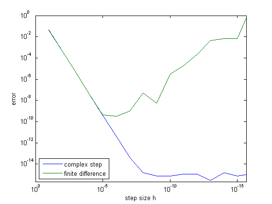
This confirms that complex step is accurate for small step sizes whereas the finite difference approach never achieves full accuracy.
References
Lyness, James N., and Moler, Cleve B., Numerical Differentiation of Analytic Functions, SIAM J. Numerical Analysis 4, 1967, pp. 202-210. epubs.siam.org/doi/abs/10.1137/0704019
Squire, William, and Trapp, George, Using complex variables to estimate derivatives of real functions, SIAM Review 40, 1998, pp. 110-112. epubs.siam.org/doi/abs/10.1137/S003614459631241X
Martins, Joaquim R. R. A., Sturdza, Peter, and Alonso, Juan J., The Complex-Step Derivative Approximation, ACM Transactions on Mathematical Software 29, 2003, pp. 245-262, Martins2003CSD.pdf
Martins, Joaquim R. R. A., A Guide to the Complex-Step Derivative Approximation, complex step guide
Kenway, Gaetan K.W., Kennedy, Graeme J., and Martins, Joaquim R. R. A., A scalable parallel approach for high-fidelity steady-state aeroelastic analysis and adjoint derivative computations, AIAA Journal (In Press)
- Category:
- Algorithms,
- Calculus,
- History,
- Numerical Analysis


Comments
To leave a comment, please click here to sign in to your MathWorks Account or create a new one.