
MATLAB History, PC-MATLAB Version 1.0
The ACM Special Interest Group on Programming Languages, SIGPLAN, expects to hold the fourth in a series of conferences on the History of Programming Languages in 2020, see HOPL-IV. The first drafts of papers are to be submitted by August, 2018. That long lead time gives me the opportunity to write a detailed history of MATLAB. I plan to write the paper in sections, which I'll post in this blog as they are available.
This is the fourth such installment. MATLAB takes the first steps from a primitive matrix calculator to a full-fledged technical computing environment.
Contents
Stanford, 1979
I spent the 1979-80 academic year at Stanford, as a Visiting Professor of Computer Science. In the fall I taught CS237a, the graduate course in Numerical Analysis. I introduced the class to the matrix calculator that I called Historic MATLAB in my previous post about MATLAB history.
There were maybe fifteen to twenty students in the class. About half of them were Math and CS students. As I remember, they were not impressed with MATLAB. It was not a particularly sophisticated programming language. It was not numerical analysis research.
But the other half of the students were from engineering at Stanford. They loved MATLAB. They were studying subjects like control theory and signal processing that, back then, I knew nothing about. Matrices were a central part of the mathematics in these subjects. The students had been doing small matrix problems by hand and larger problems by writing Fortran programs. MATLAB was immediately useful.
Jack Little
Jack Little studied electrical engineering at MIT in the late 1970's and then came west to Stanford for grad school. He didn't take my CS237 course, but a friend of his did. The friend showed him MATLAB and Little immediately adopted it for his own work in control systems and signal processing.
In 1983 Little suggested the creation of a commercial product based on MATLAB. I said I thought that was a good idea, but I didn't join him initially. The IBM PC had been introduced only two years earlier and was barely powerful enough to run something like MATLAB, but Little anticipated its evolution. He left his job, bought a Compaq PC clone at Sears, moved into the hills behind Stanford, and, with my encouragement, spent a year and a half creating a new and extended version of MATLAB written in C. A friend, Steve Bangert, joined the project and worked on the new MATLAB in his spare time.
MathWorks
The three of us -- Little, Bangert, and myself -- formed MathWorks in California in 1984. PC-MATLAB made its debut in December 1984 at the IEEE Conference on Decision and Control in Las Vegas.
Little and Bangert made many important modifications and improvements to Historic MATLAB when they created the new and extended version. The most significant were functions, toolboxes and graphics
Functions
The MATLAB function naming mechanism uses the underlying computer file system. A script or function is a body of MATLAB code stored in a file with the extension .m. If the file begins with the keyword function, then it is a function, otherwise it is a script. The name of the file, minus the .m, is the name of the script or function. For example, a file named hello.m containing the single line
disp('Hello World')is a MATLAB script. Typing the file name without the .m extension at the command line produces the traditional greeting.
hello
Hello World
Functions usually have input and output arguments. Here is a simple example that uses a vector outer product to generate the multiplication table you memorized in elementary school
type mults
function T = mults(n)
    j = 1:n;
    T = j'*j;
end
This statement produces a 10-by-10 multiplication table.
T = mults(10)
T =
     1     2     3     4     5     6     7     8     9    10
     2     4     6     8    10    12    14    16    18    20
     3     6     9    12    15    18    21    24    27    30
     4     8    12    16    20    24    28    32    36    40
     5    10    15    20    25    30    35    40    45    50
     6    12    18    24    30    36    42    48    54    60
     7    14    21    28    35    42    49    56    63    70
     8    16    24    32    40    48    56    64    72    80
     9    18    27    36    45    54    63    72    81    90
    10    20    30    40    50    60    70    80    90   100
Input arguments to MATLAB functions are "passed by value" or, more precisely, passed by "copy on write". It is not necessary to make copy of an input argument if the function does not change it. For example, the function
  function C = commuator(A,B)
     C = A*B - B*A;
  end
does not change A or B, so it does not copy either.
Toolboxes
Toolboxes are collections of functions written in MATLAB that can be read, examined, and possibly modified, by users. The matlab toolbox, which is an essential part of every installation, has several dozen functions that provide capabilities beyond the built-in functions in the core.
Other toolboxes are available from MathWorks and many other sources. The first two specialized toolboxes were control and signal.
Graphics
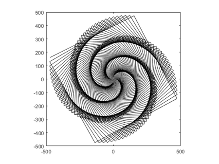
Technical computer graphics have been an essential part of MATLAB since the first MathWorks version. Let's look at two examples from that first version. Notice that neither one has anything to do with numerical linear algebra, but they both rely on vector notation and array operations. One demo was called simply wow.
type wow
% Lets define a peculiar vector, and then plot
% a growing cosine wave versus a growing sine:

    t = 0:(.99*pi/2):500;
    x = t.*cos(t);
    y = t.*sin(t);
    plot(x,y,'k')
    axis square
wow
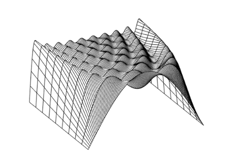
The second example investigates the Gibbs phenomena by plotting the successive partial sums of the Fourier series for a square wave.
type square_wave
%	For a finale, we can go from the fundamental to the 19th harmonic
%	and create vectors of successively more harmonics, saving all
%	intermediate steps as rows in a matrix.

    t = 0:pi/128:pi;
    y = zeros(10,max(size(t)));
    x = sin(t);
    y(1,:) = x;
    i = 1;

    for k = 3:2:19
        i = i + 1;
        x = x + sin(k*t)/k;
        y(i,:) = x;
    end

%	We can plot these successively on an overplot, showing the transition
%	to a square wave.  Note that Gibb's effect says that you will never
%	really get there.
%	Or we can plot this as a 3-d mesh surface.

    mesh(y)
    colormap([0 0 0])  % Black and white.
    axis tight
    axis off
    view([-27 39])
square_wave
Contents
I cannot find a disc for the very first version of PC-MATLAB. The oldest I can find is version 1.3. Here are all the functions, key words, and operators in that version.
Information and assistance:
help   - help facility (help intro, help index)
demo   - run demonstrations
browse - browse utility
who    - lists current variables in memory
what   - lists .M files on disk
dir    - directory list of files on disk
casesen- turn off case sensitivity
format - set output format
pack   - memory garbage collection and compaction
edit   - invoke editor
Attributes and Array Manipulation:
max     - maximum value in vector
min     - minimum value in vector
sum     - sum of elements in vector
prod    - product of elements in vector
cumsum  - cumulative sum of elements in vector
cumprod - cumulative product of elements in vector
mean	- mean value in a vector
median	- median value in a vector
std	- standard deviation in a vector
size    - row and column dimensions of an array
length  - length of a vector
:       - array subscripting, selection, and removing
sort    - sorting
find    - find array indices of logical values
hist    - histograms
Array Building Functions:
diag    - creates diagonal arrays, removes diagonal vectors
eye     - creates identity matrices
ones    - generates an array of all ones
zeros   - generates an array of all zeros
rand    - random numbers and arrays
magic   - generates a magic square
tril    - lower triangular part
triu    - upper triangular part
hilb    - generates Hilbert matrix
invhilb - generates inverse Hilbert matrix
Matrix Properties:
cond  - condition number in 2-norm
det   - determinant
norm  - 1-norm, 2-norm, F-norm, infinity norm
rank  - rank
rcond - condition estimate
Matrix Functions:
inv   - inverse
expm  - matrix exponential
logm  - matrix logarithm
sqrtm - matrix square root
funm  - arbitrary matrix functions
pinv  - pseudoinverse
poly  - characteristic polynomial
kron  - Kronecker tensor product
Matrix Decompositions and Factorizations:
chol  - Cholesky factorization
eig   - eigenvalues and eigenvectors
hess  - Hessenberg form
lu    - factors from Gaussian elimination
orth  - orthogonalization
qr    - orthogonal-triangular decomposition
schur - Schur decomposition
svd   - singular value decomposition
Polynomial manipulations:
poly    - characteristic polynomial
roots   - find polynomial roots
polyval - evaluate polynomial
conv  	- multiplication
Signal Processing:
filter - digital filter
fft    - fast Fourier transform
ifft   - inverse fast Fourier transform
conv   - convolution
length - length of a sequence
Permanent Variables:
ans     - answer when expression is not assigned
eps     - machine epsilon, floating point relative accuracy
pi      - 3.14159265358979323846264338327950288419716939937511...
inf     - infinity
nan     - Not-a-Number
nargin  - number of input arguments in a function
nargout - number of output arguments in a function
Control Flow:
if s		  conditionally execute statements
 elseif s
 else
end
for i=v,.. end    repeat statements a specific number of times
while s,..,end    do while
break             break out of a for or while loop
return            return from function
Graphics and Plotting:
shg    - show graphics screen
cla    - clear alpha screen
clg    - clear graphics screen
plot   - linear X-Y plot
loglog - loglog X-Y plot
semilogx - semi-log X-Y plot
semilogy - semi-log X-Y plot
polar  - polar plot
mesh   - 3-dimensional mesh surface
title  - plot title
xlabel - x-axis label
ylabel - y-axis label
grid   - draw grid lines
axis   - manual axis scaling
print  - hardcopy
disp   - compact matrix display
User-defined Functions, Procedures, and Programming:
type    - list a Function or file
what    - lists .M files on disk
input   - get a number from the user
pause   - pause until <cr> entered
return  - return from a user defined Function
eval    - interpret text in a variable
setstr  - set flag indicating matrix is a string
echo    - enables command echoing
nargin  - number of input arguments in a function
nargout - number of output arguments in a function
exist	- checks if a variable or function exists
Disk Files:
diary  - diary of the session in a disk file
load   - loads variables from a file
save   - saves variables on a file
type   - list a file
dir    - directory list of files on disk
delete - delete files
chdir  - change working directory
Elementary Math Functions:
abs   - absolute value or complex magnitude
conj  - complex conjugate
fix   - round towards zero
imag  - imaginary part
real  - real part
round - round to nearest integer
sign  - signum function
sqrt  - square root
rem   - remainder
sin, cos, tan
asin, acos, atan
atan2  - four quadrant arctangent
exp    - exponential base e
log    - natural logarithm
log10  - log base 10
bessel - Bessel functions
rat    - rational number approximation
Special Symbols:
=  - assignment statement
[  - used to form vectors and matrices
]  - see [
(  - arithmetic expression precedence
)  - see (
.  - Decimal point
.. - continue a statement to the next line
,  - separates matrix subscripts and function arguments
;  - Ends rows. Suppresses the display of a variable
%  - comment statement
:  - subscripting, vector generation, data selection
'  - transpose, string delimiter
Element-by-element arithmetic operators:
+  - addition
-  - subtraction
.*  - multiplication
./  - division
.\  - left division
.^  - raise to a power
.'  - transpose
Matrix operators:
*  - multiplication
/  - division
\  - left division
^  - raise to a power
'  - matrix conjugate transpose
Relational operators:
<  - less than
<= - less than or equals
>  - greater than
>= - greater than or equals
== - equals
~= - not equals
Logical operators:
+  - OR
.* - AND
~  - NOT (complement)


Comments
To leave a comment, please click here to sign in to your MathWorks Account or create a new one.