 Cleve’s Corner: Cleve Moler on Mathematics and Computing
 The MATLAB Blog
 Guy on Simulink
 MATLAB Community
 Artificial Intelligence
 Developer Zone
 Stuart’s MATLAB Videos
 Behind the Headlines
 File Exchange Pick of the Week
 Hans on IoT
 Student Lounge
 MATLAB ユーザーコミュニティー
 Startups, Accelerators, & Entrepreneurs
 Autonomous Systems
 Quantitative Finance
 MATLAB Graphics and App Building
Reviving Wilson’s Matrix
I probably first saw this matrix in 1960 in John Todd's class at Caltech. But I forgot about it until Tahar Loulou jogged my memory with a comment following my blog post in late May. It deserves a place in our gallery of interesting matrices.
Contents
T. S. Wilson
I'm afraid that I don't know very much about T. S. Wilson himself. The only paper we could find on the Internet is the joint paper about pendulum dampers listed in the references. This paper, which does not mention the matrix, was published in 1940. The authors were from a British company called D. Napier & Son Ltd. The earliest appearance of the matrix that we know of is the 1946 paper by J. Morris referenced below. It is possible that by this time Wilson and Morris were colleagues at the Royal Aircraft Establishment in Farnborough in the UK.
I think that Wilson and Todd must have known each other. Todd acknowledges Wilson in several papers and books.
One of the references we used in Todd's class is the booklet written by Marvin Marcus also referenced below. The booklet has a short section collecting some "particular" matrices. A_13 is our old friend the Hilbert matrix and A_14 is Wilson's matrix.
T. S. Wilson's Matrix
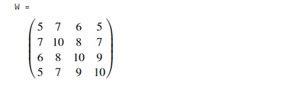
Here is the matrix. Let's use the Live Editor® and the Symbolic Math Toolbox®.
W = sym([5 7 6 5; 7 10 8 7; 6 8 10 9; 5 7 9 10]);
Determinant and Inverse
The first noteworthy property is the determinant. The determinant has to be an integer because all the matrix elements are integers.
d = det(W);

This is the smallest possible determinant for a nonsingular matrix with integer entries.
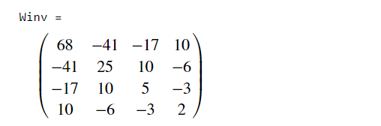
Since the determinant is one, the inverse must also have integer entries.
Winv = round(inv(W));
Cholesky
The matrix is symmetric. Let's use chol to verify that it is positive definite.
    try
        R = chol(W);
    catch
        disp("Not SPD.")
    end
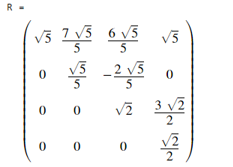
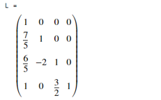
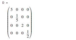
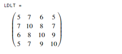
Since chol was successful we know that W is positive definite. Factor out the diagonal to get a nice rational $LDL^T$ factorization.
    D = diag(diag(R));
    L = R'/D;
    D = D^2;
    LDLT = L*D*L';
Eigenvalues
The characteristic polynomial is a quartic with integer coefficients.
p = charpoly(W,'lambda');

Since the degree of p is less than 5, the exact eigenvalues can be expressed in closed form.
e = eig(W);
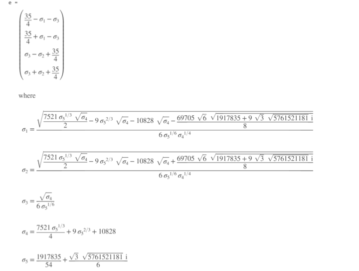
We asked for it. Like it or not, that's the exact answer. Since p does not factor nicely over the rationals, the closed form is intimidating. It's hard to tell which eigenvalue is the largest, for example. Notice that even though the eigenvalues are real, the formulae involve complex numbers whose imaginary parts necessarily cancel.
For the remainder of this article, let's revert to floating point arithmetic.
W = double(W)
W =
     5     7     6     5
     7    10     8     7
     6     8    10     9
     5     7     9    10
Now the computed eigenvalues are approximate, but more useful.
e = eig(W)
e =
    0.0102
    0.8431
    3.8581
   30.2887
Condition
Is this matrix poorly conditioned?
condW = cond(W)
condW =
   2.9841e+03
So the condition is "only" about 3000. That may not seem to be very badly conditioned. But let's look more closely. Set up a linear system where we know the exact solution.
   xact = ones(4,1);
   b = W*xact
b =
    23
    32
    33
    31
And solve it.
x = W\b
x =
    1.0000
    1.0000
    1.0000
    1.0000
We expect to get all ones, and we do. But now perturb the right-hand side a little.
   delta_b = [.01 -.01 .01 -.01]'
   b_prime = b + delta_b
delta_b =
    0.0100
   -0.0100
    0.0100
   -0.0100
b_prime =
   23.0100
   31.9900
   33.0100
   30.9900
This perturbation changes the solution drastically.
x_prime = W\b_prime
x_prime =
    1.8200
    0.5000
    0.8100
    1.1100
An Experiment
I want to argue that Wilson's matrix is badly conditioned, when compared to matrices with these properties.
- 4-by-4
- Symmetric
- Nonsingular
- Integer entries between 1 and 10.
My experiment involves generating one million random matrices with these properties. Random symmetric matrices are created by
    U = triu(randi(10,4,4));
    A = U + triu(U,1)';
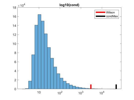
One typical run produced these statistics.
- Number of matrices = 1000000
- Singular = 1820
- Positive definite = 11217
- Condition > condW = 2115
- Maximum condition = 4.8087e4
The distribution of the condition numbers looks like this. We can see that Wilson's matrix is unusual. Only about 0.21 percent of comparable matrices have a larger condition number.
By the way, the matrix with the largest condition number in this run was
condMax
condMax =
     1     3    10    10
     3     4     8     9
    10     8     3     9
    10     9     9     3
Thanks
Thanks to Tahar Loulou whose comment got this all started, to Steve Lord who contributed another comment, and to Jan Peter Schäfermeyer, Nick Higham and Sven Hammarling for their email pointing to references.
References
R. W. Zdanowich and T. S. Wilson, "The elements of pendulum dampers," Proceedings of the Institution of Mechanical Engineers, 143_028_02, pp. 182-210, 1940, link.
J. Morris, "XVI. An escalator process for the solution of linear simultaneous equations", The London, Edinburgh, and Dublin Philosophical Magazine and Journal of Science, 37:265, pp. 106-120, 1946, link.
Jacques Delforge, "Application of the concept of the conditioning of a matrix to an identification problem," Comp. and Maths with Appls., Vol. 4, pp. 139-148, 1978, link.
E. Bodewig, Matrix calculus, North Holland, Amsterdam, 2nd edition, 1959.
John Todd, "The condition of a certain matrix," Proceedings of the Cambridge Philosophical Society, vol. 46, pp. 116-118, 1950, link.
John Todd, Basic Numerical Algorithms: Vol. 2: Numerical Algorithms, Birkhäuser Verlag, Basel, 1977.
Marvin Marcus, Basic Theorems in Matrix Theory, National Bureau of Standards, Applied Mathematics Series, number 57, page 22, 1960, link.
- Category:
- History,
- Matrices,
- Numerical Analysis,
- People


Comments
To leave a comment, please click here to sign in to your MathWorks Account or create a new one.