
A Matrix for the New HPL-AI Benchmark
My colleagues are looking for a matrix to be used in a new benchmark. They've come to the right place.
Contents
A couple of weeks ago I got this email from Jack Dongarra at the University of Tennessee.
For this new HPL-AI benchmark, I'm looking for a matrix that is not symmetric, is easily generated (roughly O(n^2) ops to generate), is dense, doesn’t require pivoting to control growth, and has a smallish condition number (<O(10^5)).
There are two steps for the benchmark:
1) do LU on the matrix in short precision and compute an approximation solution x. (On Nvidia this is 6 times faster in half precision then in DP.)
2) do GMRES on with L and U as preconditions with x as the starting point (this usually takes 3-4 iterations to converge.)
The benchmark details are here: http://bit.ly/hpl-ai.
Any ideas for a matrix?
Symmetric Hilbert Matrix
One of the first matrices I ever studied was the Hilbert matrix. With the singleton expansion features now in MATLAB, the traditional symmetric Hilbert matrix can be generated by
  format rat
  n = 5;
  i = 1:n
  j = i'
  H = 1./(i+j-1)
i =
       1              2              3              4              5
j =
       1
       2
       3
       4
       5
H =
       1              1/2            1/3            1/4            1/5
       1/2            1/3            1/4            1/5            1/6
       1/3            1/4            1/5            1/6            1/7
       1/4            1/5            1/6            1/7            1/8
       1/5            1/6            1/7            1/8            1/9
When you add the row vector i to the column vector j, the resulting i+j is a matrix. Compare this with the inner product, i*j, which produces a scalar, and the outer product, j*i, which produces another matrix. The expression i+j can be thought of as an "outer sum".
Two more scalar expansions complete the computation; i+j-1 subtracts 1 from each element of the sum and 1./(i+j-1) divides 1 by each element in the denominator. Both of these scalar expansions have been in MATLAB from its earliest days.
The elements of Hilbert matrices depend only on the sum i+j, so they are constant on the antidiagonals. Such matrices are known as Cauchy matrices. There are fast algorithms for solving system of equations involving Cauchy matrices in $O(n^2)$ time.
Nonsymmetric Hilbert Matrix
Some years ago, I wanted a nonsymmetric test matrix, so I changed the plus sign in the denominator of the Hilbert matrix to a minus sign. But this created a division by zero along the subdiagonal, so I also changed the -1 to +1/2. I call this the "nonsymmetric Hilbert matrix."
H = 1./(i-j+1/2)
H =
       2              2/3            2/5            2/7            2/9
      -2              2              2/3            2/5            2/7
      -2/3           -2              2              2/3            2/5
      -2/5           -2/3           -2              2              2/3
      -2/7           -2/5           -2/3           -2              2
The elements depend only on i-j and so are constant on the diagonals. The matrices are Toeplitz and, again, such systems can be solved with $O(n^2)$ operations.
I was astonished when I first computed the singular values of nonsymmetric Hilbert matrices -- most of them were nearly equal to $\pi$. Already with only the 5-by-5 we see five decimal places.
   format long
   sigma = svd(H)
sigma =
   3.141589238341321
   3.141272220456508
   3.129520593545258
   2.921860834913688
   1.461864493324889
This was a big surprise. The eventual explanation, provided by Seymour Parter, involves a theorem of Szego from the 1920's relating the eigenvalues of Toeplitz matrices to Fourier series and square waves.
Benchmark Matrix
I have been working with Jack's colleague Piotr Luszczek. This is our suggestion for the HPL-AI Benchmark Matrix. It depends upon two parameters, n and mu. As mu goes from 1 to -1, the core of this matrix goes from the symmetric to the nonsymmetric Hilbert matrix. Adding n in the denominator and 1's on the diagonal produces diagonal dominance.
A = 1./(i + mu*j + n) + double(i==j);
   clear A
   type A
function Aout = A(n,mu)
% A(n,mu).  Matrix for the HPL-AI Benchmark.  mu usually in [-1, 1].
    i = 1:n;
    j = i';
    Aout = 1./(i+mu*j+n) + eye(n,n);
end
If mu is not equal to +1, this matrix is not Cauchy. And, if mu is not equal to -1, it is not Toeplitz. Furthermore, if mu is greater than -1, it is diagonally dominant and, as we shall see, very well-conditioned.
Example
Here is the 5x5 with rational output. When mu is +1, we get a section of a symmetric Hilbert matrix plus 1's on the diagonal.
   format rat
   mu = 1;
   A(n,mu)
ans =
       8/7            1/8            1/9            1/10           1/11
       1/8           10/9            1/10           1/11           1/12
       1/9            1/10          12/11           1/12           1/13
       1/10           1/11           1/12          14/13           1/14
       1/11           1/12           1/13           1/14          16/15
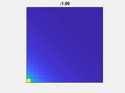
And when mu is -1, the matrix is far from symmetric. The element in the far southwest corner almost dominates the diagonal.
   mu = -1;
   A(n,mu)
ans =
       6/5            1/6            1/7            1/8            1/9
       1/4            6/5            1/6            1/7            1/8
       1/3            1/4            6/5            1/6            1/7
       1/2            1/3            1/4            6/5            1/6
       1              1/2            1/3            1/4            6/5
Animation
Here is an animation of the matrix without the addition of eye(n,n). As mu goes to -1 to 1, A(n,mu)-eye(n,n) goes from nonsymmetric to symmetric.
Gaussian elimination
If mu > -1, the largest element is on the diagonal and lu(A(n,mu)) does no pivoting.
   format short
   mu = -1
   [L,U] = lu(A(n,mu))

   mu = 1
   [L,U] = lu(A(n,mu))
mu =
    -1
L =
    1.0000         0         0         0         0
    0.2083    1.0000         0         0         0
    0.2778    0.1748    1.0000         0         0
    0.4167    0.2265    0.1403    1.0000         0
    0.8333    0.3099    0.1512    0.0839    1.0000
U =
    1.2000    0.1667    0.1429    0.1250    0.1111
         0    1.1653    0.1369    0.1168    0.1019
         0         0    1.1364    0.1115    0.0942
         0         0         0    1.1058    0.0841
         0         0         0         0    1.0545
mu =
     1
L =
    1.0000         0         0         0         0
    0.1094    1.0000         0         0         0
    0.0972    0.0800    1.0000         0         0
    0.0875    0.0729    0.0626    1.0000         0
    0.0795    0.0669    0.0580    0.0513    1.0000
U =
    1.1429    0.1250    0.1111    0.1000    0.0909
         0    1.0974    0.0878    0.0800    0.0734
         0         0    1.0731    0.0672    0.0622
         0         0         0    1.0581    0.0542
         0         0         0         0    1.0481
Condition
Let's see how the 2-condition number, $\sigma_1/\sigma_n$, varies as the parameters vary. Computing the singular values for all the matrices in the following plots takes a little over 10 minutes on my laptop.
sigma_1
   load HPLAI.mat s1 sn n mu

   surf(mu,n,s1)
   view(25,12)
   xlabel('mu')
   ylabel('n')
   set(gca,'xlim',[-0.9 1.0], ...
       'xtick',[-0.9 -0.5 0 0.5 1.0], ...
       'ylim',[0 2500])
   title('\sigma_1')
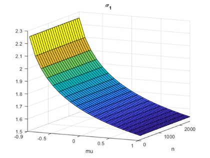
The colors vary as mu varies from -0.9 up to 1.0. I am staying away from mu = -1.0 where the matrix looses diagonal dominance. The other horizontal axis is the matrix order n. I have limited n to 2500 in these experiments.
The point to be made is that if mu > -0.9, then the largest singular value is bounded, in fact sigma_1 < 2.3.
sigma_n
   surf(mu,n,sn)
   view(25,12)
   xlabel('mu')
   ylabel('n')
   set(gca,'xlim',[-0.9 1.0], ...
       'xtick',[-0.9 -0.5 0 0.5 1.0], ...
       'ylim',[0 2500])
   title('\sigma_n')
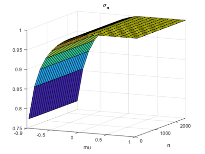
If mu > -0.9, then the smallest singular value is bounded away from zero, in fact sigma_n > .75.
sigma_1/sigma_n
   surf(mu,n,s1./sn)
   view(25,12)
   xlabel('mu')
   ylabel('n')
   set(gca,'xlim',[-0.9 1.0], ...
       'xtick',[-0.9 -0.5 0 0.5 1.0], ...
       'ylim',[0 2500])
   title('\sigma_1/\sigma_n')

If mu > -0.9, then the condition number in the 2-norm is bounded, sigma_1/sigma_n < 2.3/.75 $\approx$ 3.0 .
Overflow
The HPL-AI benchmark would begin by computing the LU decomposition of this matrix using 16-bit half-precision floating point arithmetic, FP16. So, there is a signigant problem if the matrix order n is larger than 65504. This value is realmax, the largest number that can be represented in FP16. Any larger value of n overflows to Inf.
Some kind of scaling is going to have to be done for n > 65504. Right now, I don't see what this might be.
The alternative half-precision format to FP16 is Bfloat16, which has three more bits in the exponent to give realmax = 3.39e38. There should be no overflow problems while generating this matrix with Bfloat16.
Thanks
Thanks to Piotr Luszczek for working with me on this. We have more work to do.


See Also
-

Hilbert Matrices
Blogs
-

Hilbert Matrices
Blogs


评论
要发表评论,请点击 此处 登录到您的 MathWorks 帐户或创建一个新帐户。