The QR decomposition provides an estimate of the matrix condition number.

Contents

Query

Professor Magdy Hanna of the Department of Engineering Mathematics and Physics at Fayoum University in Fayoum, Egypt, asked me:

  If we have the QR decomposition of a matrix, with or without
  pivoting, is there an easy way to get the condition number of
  the matrix without starting from scratch and using the SVD?

Short answer

The short answer to Prof. Hanna's question is:

  Yes.  The ratio of the largest and smallest diagonal elements
  of qr(A) is often a good estimate of cond(A).

Compare this estimate to the exact condition of a magic square. Produce a score measuring how well the estimate does.

     A = magic(11);
     R = qr(A);
     d = abs(diag(R));
     est = max(d)/min(d);
     kappa = cond(A);
     disp("       est     kappa     score")
     disp([est kappa est/kappa])

 

       est     kappa     score
    2.6964   11.1021    0.2429

QR Decomposition

A more complete answer involves column pivoting.

The QR decomposition without column pivoting is an orthogonal Q and an upper triangular R so that

  A = Q*R

The QR composition with column pivoting is an orthogonal Q, an upper triangular R and a permutation P that reorders the columns of A so that

  A*P = Q*R

In either case, Q and P are orthogonal, so

  cond(R) = cond(A)

Any estimate of the condition of R provides an estimate of the condition of A.

tricond

An estimate the condition of a triangular matrix is the ratio of the largest and smallest elements on the diagonal.

   type tricond

     function cond = tricond(T)
        % Estimate condition of lower or upper triangular matrix.
        if istril(T) || istriu(T)
            D = diag(abs(T));
            cond = max(D)/min(D);
        else
            cond =  NaN;
        end
     end

qr function

Here is the 4-by-4 Pascal matrix

    A = pascal(4)

A =

     1     1     1     1
     1     2     3     4
     1     3     6    10
     1     4    10    20

This matrix is reasonably well conditioned.

    kappa = cond(A)

kappa =

  691.9374

With one output, the qr function provides the "Q-less" QR decomposition with no pivoting.

(With two outputs, the qr function produces the same R and also reveals the orthogonal Q.)

    R = qr(A)

R =

   -2.0000   -5.0000  -10.0000  -17.5000
         0   -2.2361   -6.7082  -14.0872
         0         0    1.0000    3.5000
         0         0         0   -0.2236

For this matrix tricond without pivoting produces a poor estimate of the exact condition.

    trico = tricond(R);
    kappa = cond(A);
    disp("   tricond     kappa     score")
    disp([trico kappa trico/kappa])

  

   tricond     kappa     score
   10.0000  691.9374    0.0145

With three outputs, qr does column pivoting and returns a different R.

    [Q,R,P] = qr(A);
    R

R =

  -22.7376   -5.2336   -1.5393  -12.0065
         0   -1.6153   -1.2034   -1.3387
         0         0    0.4270   -0.2170
         0         0         0   -0.0638

Compare tricond and the exact condition.

    trico = tricond(R);
    disp("   tricond     kappa     score")
    disp([trico kappa trico/kappa])

 

   tricond     kappa     score
  356.6259  691.9374    0.5154

Column pivoting produces a much better tricond estimate for this matrix.

Gallery

Let's do more tests using these matrices from the MATLAB Gallery.

    funs = ["moler", "parter", "binomial",  "chebspec", "cauchy",...
           "chebspec", "chebvand","circul", "frank", "ris"];

One of these Gallery matrices is the "moler" matrix, even though I didn't invent it. A precursor to the "moler" matrix is a badly conditioned upper triangular matrix with ones on the diagonal, minus ones above the diagonal and zeros below.

    n = 5;
    U = eye(n) - triu(ones(n),1)

U =

     1    -1    -1    -1    -1
     0     1    -1    -1    -1
     0     0     1    -1    -1
     0     0     0     1    -1
     0     0     0     0     1

The "moler" matrix is

    M = U'*U

M =

     1    -1    -1    -1    -1
    -1     2     0     0     0
    -1     0     3     1     1
    -1     0     1     4     2
    -1     0     1     2     5

The "moler" matrix squares the condition of U. The condition of M grows like 4^n.

    kappa = cond(M)

kappa =

  865.9801

The tricond score without column pivoting is very poor.

    R = qr(M);
    trico = tricond(R);
    disp("   tricond     kappa     score")
    disp([trico kappa trico/kappa])

 

   tricond     kappa     score
   20.7364  865.9801    0.0239

With pivoting the score is much better.

    [~,R,~] = qr(M);

    trico = tricond(R);
    disp("   tricond     kappa     score")
    disp([trico kappa trico/kappa])

  

  tricond     kappa     score
  555.0198  865.9801    0.6409

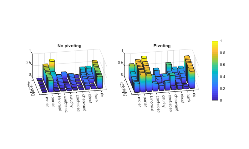
These scores are in the first line of the following output and in the upper left-hand corners of the 3-D bar graphs.

Tests

   [Dnopiv,Dpiv,xt,yt] = tester(funs);

         fun     n    nopiv    piv


       moler     5    0.024    0.641 
                10    0.000    0.426 
                15    0.000    0.337 
                20    0.000    0.287 
                25    0.000    0.372 

      parter     5    0.610    0.804 
                10    0.564    0.776 
                15    0.536    0.757 
                20    0.517    0.744 
                25    0.502    0.735 

    binomial     5    0.795    0.926 
                10    0.387    0.817 
                15    0.150    0.768 
                20    0.056    0.696 
                25    0.021    0.674 

    chebspec     5    0.120    0.110 
                10    0.236    0.095 
                15    0.183    0.358 
                20    0.132    0.165 
                25    0.022    0.318 

      cauchy     5    0.217    0.376 
                10    0.034    0.242 
                15    0.016    0.247 
                20    0.058    0.116 
                25    0.102    0.222 

    chebspec     5    0.120    0.110 
                10    0.236    0.095 
                15    0.183    0.358 
                20    0.132    0.165 
                25    0.022    0.318 

    chebvand     5    0.055    0.577 
                10    0.002    0.326 
                15    0.000    0.338 
                20    0.000    0.492 
                25    0.000    0.082 

      circul     5    0.370    0.370 
                10    0.252    0.252 
                15    0.209    0.209 
                20    0.180    0.180 
                25    0.162    0.162 

       frank     5    0.390    0.390 
                10    0.257    0.296 
                15    0.191    0.248 
                20      Inf    0.013 
                25    0.039    0.100 

         ris     5    0.610    0.804 
                10    0.564    0.776 
                15    0.536    0.757 
                20    0.517    0.744 
                25    0.502    0.735 

Plot

   [c,ax1,ax2] = ploter(funs,Dnopiv,Dpiv,xt,yt);

Published with MATLAB® R2026a