Solving Ordinary Differential Equations

I have recently handled several help requests for solving differential equations in MATLAB. All of the cases I worked on boil down to how to transform the higher-order equation(s) given to a system of first order equations. In this post I will outline how to accomplish this task and solve the equations in question. What I am not going to talk about is details of ODE solving algorithms (maybe another time).

Contents

Simple System

Let's start with a simple, linear, second order system, a mass-spring system with motion constrained to one-dimension, a horizontal one (and therefore no gravity). If is the mass and is the spring constant, the equations of motion for the system are:

Conditions, Initial and Otherwise

To solve this system, we need to know , , , and initial conditions, e.g., (also known as position and velocity). Let's simplify things and set , i.e., no external forces. Let's also set some initial conditions, , in other words, start with the spring unstretched and the mass moving. I end up with this system:

Transform Equation

Looking in the help, I need to set up an system of equations to enable me to use one of the numerical ODE solvers in MATLAB.

To start the transformation, let me define a new variable that I will substitute in the system.

I can derive

and now rewrite my ODE system in terms of .

with initial conditions as above.

Now let me reorganize these 2 equations in a vector/matrix equation where

I now write me equation solely in terms of , the new vector (consisting of position and velocity). With that in mind, I will reorganize the existing equations first so I have on the left-hand sides.

or, in terms of ,

Try It!

Let's try it. Set values for m and k

m = 1;
k = 10;

I can create the ODE code in a file, or I can set up the equations as an anonymous function which is what I'll do here.

springmass = @(t,z)[z(2); -k * z(1)/ m];

Set up the initial conditions.

ic = [0; 1];

Solve between .

tspan = [0 10];

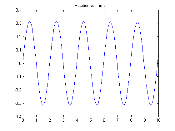
Call an ODE solver and plot the results.

[t,y] = ode23(springmass, tspan, ic);
plot(t,y(:,1)), title('Position vs. Time')

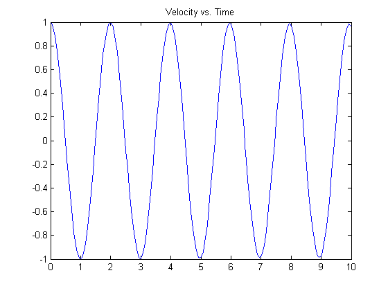
And the velocity.

plot(t,y(:,2)), title('Velocity vs. Time')

You can see the left-most points on the plots match the initial conditions specified.

Transforming Equations

Do you need to recast problems to fit into a particular formulation such as for solving ODEs? Let's hear about them here.

Get the MATLAB code

Published with MATLAB® 7.10