 Cleve’s Corner: Cleve Moler on Mathematics and Computing
 The MATLAB Blog
 Guy on Simulink
 MATLAB Community
 Artificial Intelligence
 Developer Zone
 Stuart’s MATLAB Videos
 Behind the Headlines
 File Exchange Pick of the Week
 Hans on IoT
 Student Lounge
 MATLAB ユーザーコミュニティー
 Startups, Accelerators, & Entrepreneurs
 Autonomous Systems
 Quantitative Finance
 MATLAB Graphics and App Building
Introduction to the New MATLAB Data Types for Dates and Time
Today I'd like to introduce a guest blogger, Andrea Ho, who works for the MATLAB Documentation team here at MathWorks. Today, Andrea will discuss three new data types for representing dates and times in MATLAB in R2014b - datetime, duration, and calendarDuration.
Contents
Why New Data Types?
Dates and times are frequently a critical part of data analysis. If they are part of your work, you've likely encountered some of the following limitations of date numbers, date vectors, and date strings:
- Serial date numbers are useful for numeric calculations, but they are difficult to interpret or debug.
- Date vectors and strings clearly communicate dates and times in a human-readable format, but they are not useful for calculations and comparisons.
- Date numbers, date vectors, and strings that represent both points in time and lengths of time (elapsed time) are confusing. For example, does the date vector [2015 1 1 0 0 0] represent January 1, 2015 at midnight, or an elapsed time of 2015 years, 1 month, and 1 day?
Starting in R2014b, datetime, duration, and calendarDuration are data types dedicated to storing date and time data, and are easily distinguishable from numeric values. The three types differentiate between points in time, elapsed time in units of constant length (such as hours, minutes, and seconds), and elapsed time in units of flexible length (such as weeks and months). datetime, duration, and calendarDuration represent dates and times in a way that is easy to read, is suitable for computations, has much higher precision (up to nanosecond precision), and is more memory-efficient. With the new data types, you won't have to maintain or convert between different representations of the same date and time value. Work with datetime, duration, and calendarDuration much like you do with numeric types like double, using standard array operations.
Let's see the new data types in action.
datetime for Points in Time
The datetime data type represents absolute points in time such as January 1, 2015 at midnight. The datetime function can create a datetime variable from the current date and time:
t0 = datetime('now')
t0 =
   16-Jan-2015 16:24:30
or from numeric inputs:
t0 = datetime(2015,1,1,2,3,4)
t0 =
   01-Jan-2015 02:03:04
whos t0
  Name      Size            Bytes  Class       Attributes

  t0        1x1               121  datetime
If you are interested only in the time portion of t0, you can display just that.
t0.Format = 'HH:mm'
t0 =
   02:03
Changing the format of a datetime variable affects how it is displayed, but not its numeric value. Though you can no longer see the year, month and day values, that information is still stored in the variable. Let's turn the display of the date portion of t0 back on.
t0.Format = 'dd-MMM-yyyy HH:mm'
t0 =
   01-Jan-2015 02:03
By changing the display format, you can view the value of a datetime variable with up to nanosecond precision!
t0.Format = 'dd-MMM-yyyy HH:mm:ss.SSSSSSSSS'
t0 =
   01-Jan-2015 02:03:04.000000000
If you are a frequent user of date string formats, you'll recognize that some of the format specifiers for datetime are different from those for the datestr, datenum, and datevec functions.. The new format syntax allows for more options and is now consistent with the Unicode Locale Data Markup Language (LDML) standard.
Example: Calculate Driving Time
The duration data type represents the exact difference between two specific points in time. Suppose you drove overnight, leaving your home on January 1, 2015 at 11 PM, and arriving at your destination at 4:30 AM the next day. How much time did you spend on the road? (Ignore the possibility of crossing into another time zone; we'll see how datetime manages time zones in a future post.)
t0 = datetime(2015,1,1,23,0,0);
t1 = datetime(2015,1,2,4,30,0);
dt = t1-t0
dt =
   05:30:00
dt is a duration variable displayed as hours:minutes:seconds. Like datetime, a duration behaves mostly like a numeric value but displays in a format that shows time well. Let's change the format to view dt as a number of minutes.
dt.Format = 'm'
dt =
   330 mins
We can perform common arithmetic operations on date and time variables. Even though dt is currently displayed as a number of minutes, we can add or subtract a duration in any unit, including hours and seconds.
dt2 = dt - hours(1) + seconds(5)
dt2 =
   270.08 mins
Example: Verify Payment Schedule
Suppose you opened a bank account on January 1, 2014. The account pays interest monthly on the last day of each month. Let's find the first date on which interest was paid. Is there a solution that does not depend on the account opening date? The dateshift function is useful for shifting dates to the start or end of a unit of time. In our case, we will shift the account opening date to the end of the month.
t0 = datetime(2014,1,1);
t1 = dateshift(t0,'end','month')
t1 =
   31-Jan-2014
Suppose our records indicate that we received interest payments at noon. We can add this information to t1 by modifying its Hour property.
t1.Hour = 12;
Now let's create a sequence of dates to represent the next 12 payment dates. What happens if we add increments of 30 days to t1?
t = t1 + days(0:30:335)'
t =
   31-Jan-2014 12:00:00
   02-Mar-2014 12:00:00
   01-Apr-2014 12:00:00
   01-May-2014 12:00:00
   31-May-2014 12:00:00
   30-Jun-2014 12:00:00
   30-Jul-2014 12:00:00
   29-Aug-2014 12:00:00
   28-Sep-2014 12:00:00
   28-Oct-2014 12:00:00
   27-Nov-2014 12:00:00
   27-Dec-2014 12:00:00
Yikes, most of these dates don't fall on the last day of the month. A duration of 30 days, with each day being exactly 24 hours long, was not the correct step size to use. The correct step size depends on the month, since some months have 30 days, while others have 31 (or perhaps 28, or 29). What we really want to do is add a series of calendar months to t1.
t = t1 + calmonths(0:11)'
t =
   31-Jan-2014
   28-Feb-2014
   31-Mar-2014
   30-Apr-2014
   31-May-2014
   30-Jun-2014
   31-Jul-2014
   31-Aug-2014
   30-Sep-2014
   31-Oct-2014
   30-Nov-2014
   31-Dec-2014
The calmonths function creates a calendarDuration array containing calendar months. A calendarDuration value represents a flexible or non-constant amount of time such as 1 month. There is no way to know exactly how many days, hours, minutes, or seconds there are in 1 month without knowing which month of the year I am referring to. The length of a calendar month is unknown until you relate it to a specific point in time.
How many days are between each of the payment dates?
dt = caldiff(t,'days')
dt =
   28d
   31d
   30d
   31d
   30d
   31d
   31d
   30d
   31d
   30d
   31d
Each incremental calendar month represents a different number of days.
Our bank sent us a file named interest.txt that contains interest amounts for each month of the year. We can import this data interactively using the Import Tool.

Alternatively, we can use the readtable and textscan functions to read the file programmatically. Use the %D specifier to read a date or time string and specify the string format within curly braces.
T = readtable('interest.txt','Format','%{dd MMMM yyyy HH:mm}D %f')
T =
             Date              Interest
    _______________________    ________
    31 January 2014 12:00      1.93
    28 February 2014 12:00     4.28
    31 March 2014 12:00        4.82
    30 April 2014 12:00        1.23
    31 May 2014 12:00          5.89
    30 June 2014 12:00         2.26
    31 July 2014 12:00         3.84
    31 August 2014 12:00       5.82
    30 September 2014 12:00    2.51
    31 October 2014 12:00      2.99
    30 November 2014 12:00     6.17
    31 December 2014 12:00     2.65
Even though the text file contains strings, the values in the Date column of the table are not strings. They are datetime values.
If we compare our payment times with the bank's data, we'll see that they are the same.
isequal(t,T.Date)
ans =
     1
Now let's calculate the cumulative interest at the end of each month and plot the data. When using plot, working with datetime is much easier than working with serial date numbers.
c_payments = cumsum(T.Interest);
figure
plot(T.Date,c_payments)
xlabel('Date')
ylabel('Cummulative Interest Payments')
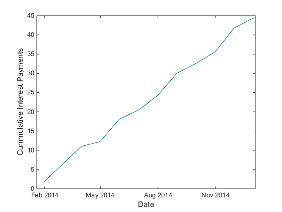
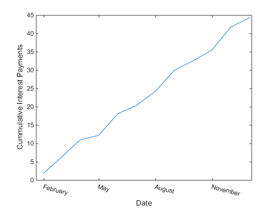
The date axis is automatically labeled with date strings that are easy to understand. You no longer have to call datetick to do this! If we want to change the format of the dates, we can specify the desired format of the axis ticks in the call to plot.
figure
plot(T.Date,c_payments,'DatetimeTickFormat','MMMM')
xlabel('Date')
ylabel('Cummulative Interest Payments')
ax = gca;
ax.XTickLabelRotation = -15;
To create charts containing date and time values using other plotting functions, you still need to work with serial date numbers for the time being. We recognize that this is inconvenient and we are planning improvements. You can learn more here about how to plot datetime and duration values.
What Else?
Notice that in our analysis of travel times and interest payments, there was no need to use serial date numbers, date vectors, or strings at all. datetime, duration, and calendarDuration allow you to manipulate dates and times quickly and more intuitively. The new data types are intended as a replacement for datenum, datevec, and datestr. However, these older functions will continue to exist in MATLAB for the foreseeable future because we know that many people rely on them in existing code.
In a future post, I'll show how datetime, duration, and calendarDuration allow you to work with time zones, daylight saving time, and dates in languages other than English.
Your Thoughts?
Do you see yourself using the new date and time data types with your data? Let us know by leaving a comment here.


댓글
댓글을 남기려면 링크 를 클릭하여 MathWorks 계정에 로그인하거나 계정을 새로 만드십시오.