
Artificial Neural Networks for Beginners
Deep Learning is a very hot topic these days especially in computer vision applications and you probably see it in the news and get curious. Now the question is, how do you get started with it? Today's guest blogger, Toshi Takeuchi, gives us a quick tutorial on artificial neural networks as a starting point for your study of deep learning.
Contents
MNIST Dataset
Many of us tend to learn better with a concrete example. Let me give you a quick step-by-step tutorial to get intuition using a popular MNIST handwritten digit dataset. Kaggle happens to use this very dataset in the Digit Recognizer tutorial competition. Let's use it in this example. You can download the competition dataset from "Get the Data" page:
- train.csv - training data
- test.csv - test data for submission
Load the training and test data into MATLAB, which I assume was downloaded into the current folder. The test data is used to generate your submissions.
tr = csvread('train.csv', 1, 0);                  % read train.csv
sub = csvread('test.csv', 1, 0);                  % read test.csv
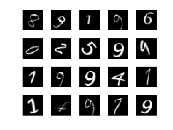
The first column is the label that shows the correct digit for each sample in the dataset, and each row is a sample. In the remaining columns, a row represents a 28 x 28 image of a handwritten digit, but all pixels are placed in a single row, rather than in the original rectangular form. To visualize the digits, we need to reshape the rows into 28 x 28 matrices. You can use reshape for that, except that we need to transpose the data, because reshape operates by column-wise rather than row-wise.
figure                                          % plot images
colormap(gray)                                  % set to grayscale
for i = 1:25                                    % preview first 25 samples
    subplot(5,5,i)                              % plot them in 6 x 6 grid
    digit = reshape(tr(i, 2:end), [28,28])';    % row = 28 x 28 image
    imagesc(digit)                              % show the image
    title(num2str(tr(i, 1)))                    % show the label
end

Data Preparation
You will be using the nprtool pattern recognition app from Deep Learning Toolbox. The app expects two sets of data:
- inputs - a numeric matrix, each column representing the samples and rows the features. This is the scanned images of handwritten digits.
- targets - a numeric matrix of 0 and 1 that maps to specific labels that images represent. This is also known as a dummy variable. Deep Learning Toolbox also expects labels stored in columns, rather than in rows.
The labels range from 0 to 9, but we will use '10' to represent '0' because MATLAB is indexing is 1-based.
1 --> [1; 0; 0; 0; 0; 0; 0; 0; 0; 0]
2 --> [0; 1; 0; 0; 0; 0; 0; 0; 0; 0]
3 --> [0; 0; 1; 0; 0; 0; 0; 0; 0; 0]
            :
0 --> [0; 0; 0; 0; 0; 0; 0; 0; 0; 1]
The dataset stores samples in rows rather than in columns, so you need to transpose it. Then you will partition the data so that you hold out 1/3 of the data for model evaluation, and you will only use 2/3 for training our artificial neural network model.
n = size(tr, 1);                    % number of samples in the dataset
targets  = tr(:,1);                 % 1st column is |label|
targets(targets == 0) = 10;         % use '10' to present '0'
targetsd = dummyvar(targets);       % convert label into a dummy variable
inputs = tr(:,2:end);               % the rest of columns are predictors

inputs = inputs';                   % transpose input
targets = targets';                 % transpose target
targetsd = targetsd';               % transpose dummy variable

rng(1);                             % for reproducibility
c = cvpartition(n,'Holdout',n/3);   % hold out 1/3 of the dataset

Xtrain = inputs(:, training(c));    % 2/3 of the input for training
Ytrain = targetsd(:, training(c));  % 2/3 of the target for training
Xtest = inputs(:, test(c));         % 1/3 of the input for testing
Ytest = targets(test(c));           % 1/3 of the target for testing
Ytestd = targetsd(:, test(c));      % 1/3 of the dummy variable for testing
Using the Deep Learning Toolbox GUI App
- You can start the Neural Network Start GUI by typing the command nnstart.
- You then click the Pattern Recognition Tool to open the Neural Network Pattern Recognition Tool. You can also usehe command nprtool to open it directly.
- Click "Next" in the welcome screen and go to "Select Data".
- For inputs, select Xtrain and for targets, select Ytrain.
- Click "Next" and go to "Validation and Test Data". Accept the default settings and click "Next" again. This will split the data into 70-15-15 for the training, validation and testing sets.
- In the "Network Architecture", change the value for the number of hidden neurons, 100, and click "Next" again.
- In the "Train Network", click the "Train" button to start the training. When finished, click "Next". Skip "Evaluate Network" and click next.
- In "Deploy Solution", select "MATLAB Matrix-Only Function" and save t the generated code. I save it as myNNfun.m.
- If you click "Next" and go to "Save Results", you can also save the script as well as the model you just created. I saved the simple script as myNNscript.m
Here is the diagram of this artificial neural network model you created with the Pattern Recognition Tool. It has 784 input neurons, 100 hidden layer neurons, and 10 output layer neurons.
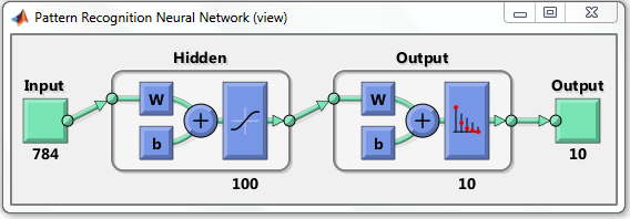
Your model learns through training the weights to produce the correct output.
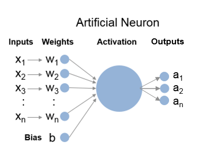
W in the diagram stands for weights and b for bias units, which are part of individual neurons. Individual neurons in the hidden layer look like this - 784 inputs and corresponding weights, 1 bias unit, and 10 activation outputs.
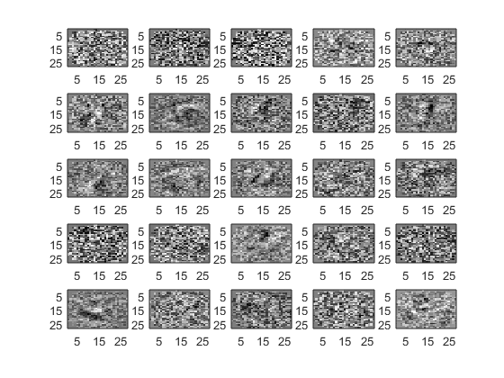
Visualizing the Learned Weights
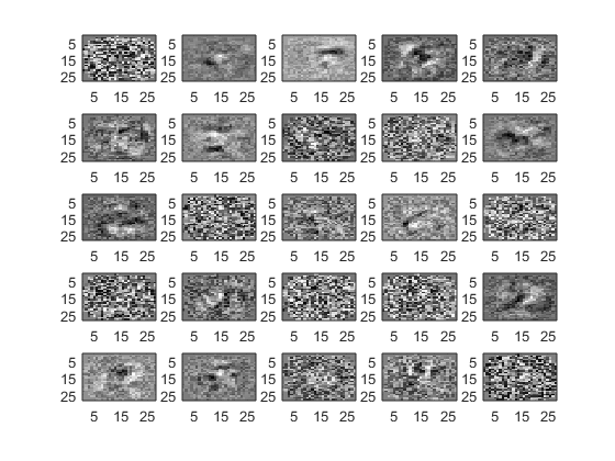
If you look inside myNNfun.m, you see variables like IW1_1 and x1_step1_keep that represent the weights your artificial neural network model learned through training. Because we have 784 inputs and 100 neurons, the full layer 1 weights will be a 100 x 784 matrix. Let's visualize them. This is what our neurons are learning!
load myWeights                          % load the learned weights
W1 =zeros(100, 28*28);                  % pre-allocation
W1(:, x1_step1_keep) = IW1_1;           % reconstruct the full matrix
figure                                  % plot images
colormap(gray)                          % set to grayscale
for i = 1:25                            % preview first 25 samples
    subplot(5,5,i)                      % plot them in 6 x 6 grid
    digit = reshape(W1(i,:), [28,28])'; % row = 28 x 28 image
    imagesc(digit)                      % show the image
end
Computing the Categorization Accuracy
Now you are ready to use myNNfun.m to predict labels for the heldout data in Xtest and compare them to the actual labels in Ytest. That gives you a realistic predictive performance against unseen data. This is also the metric Kaggle uses to score submissions.
First, you see the actual output from the network, which shows the probability for each possible label. You simply choose the most probable label as your prediction and then compare it to the actual label. You should see 95% categorization accuracy.
Ypred = myNNfun(Xtest);             % predicts probability for each label
Ypred(:, 1:5)                       % display the first 5 columns
[~, Ypred] = max(Ypred);            % find the indices of max probabilities
sum(Ytest == Ypred) / length(Ytest) % compare the predicted vs. actual
ans =
   1.3988e-09   6.1336e-05   1.4421e-07   1.5035e-07   2.6808e-08
   1.9521e-05     0.018117   3.5323e-09   2.9139e-06    0.0017353
   2.2202e-07   0.00054599     0.012391   0.00049678   0.00024934
   1.5338e-09      0.46156   0.00058973   4.5171e-07   0.00025153
   4.5265e-08      0.11546      0.91769   2.1261e-05   0.00031076
   1.1247e-08      0.25335   1.9205e-06   1.1014e-06      0.99325
   2.1627e-08    0.0045572    1.733e-08   3.7744e-07   1.7282e-07
   2.2329e-09   7.6692e-05   0.00011479      0.98698   1.7328e-06
   1.9634e-05    0.0011708     0.069215      0.01249   0.00084255
      0.99996      0.14511   1.0106e-07   2.9687e-06    0.0033565
ans =
      0.95293
Network Architecture
You probably noticed that the artificial neural network model generated from the Pattern Recognition Tool has only one hidden layer. You can build a custom model with more layers if you would like, but this simple architecture is sufficient for most common problems.
The next question you may ask is how I picked 100 for the number of hidden neurons. The general rule of thumb is to pick a number between the number of input neurons, 784 and the number of output neurons, 10, and I just picked 100 arbitrarily. That means you might do better if you try other values. Let's do this programmatically this time. myNNscript.m will be handy for this - you can simply adapt the script to do a parameter sweep.
sweep = [10,50:50:300];                 % parameter values to test
scores = zeros(length(sweep), 1);       % pre-allocation
models = cell(length(sweep), 1);        % pre-allocation
x = Xtrain;                             % inputs
t = Ytrain;                             % targets
trainFcn = 'trainscg';                  % scaled conjugate gradient
for i = 1:length(sweep)
    hiddenLayerSize = sweep(i);         % number of hidden layer neurons
    net = patternnet(hiddenLayerSize);  % pattern recognition network
    net.divideParam.trainRatio = 70/100;% 70% of data for training
    net.divideParam.valRatio = 15/100;  % 15% of data for validation
    net.divideParam.testRatio = 15/100; % 15% of data for testing
    net = train(net, x, t);             % train the network
    models{i} = net;                    % store the trained network
    p = net(Xtest);                     % predictions
    [~, p] = max(p);                    % predicted labels
    scores(i) = sum(Ytest == p) /...    % categorization accuracy
        length(Ytest);
end
Let's now plot how the categorization accuracy changes versus number of neurons in the hidden layer.
figure
plot(sweep, scores, '.-')
xlabel('number of hidden neurons')
ylabel('categorization accuracy')
title('Number of hidden neurons vs. accuracy')
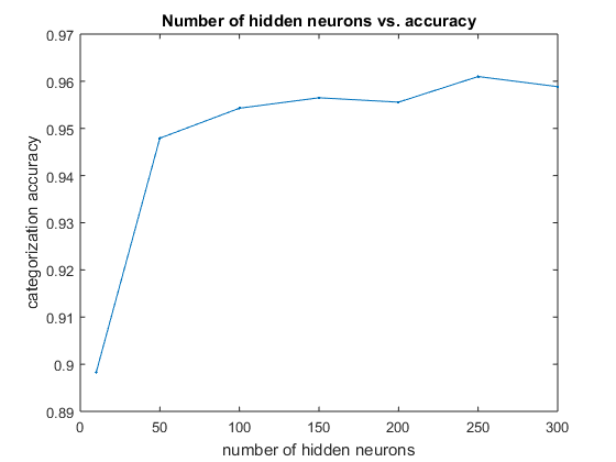
It looks like you get the best result around 250 neurons and the best score will be around 0.96 with this basic artificial neural network model.
As you can see, you gain more accuracy if you increase the number of hidden neurons, but then the accuracy decreases at some point (your result may differ a bit due to random initialization of weights). As you increase the number of neurons, your model will be able to capture more features, but if you capture too many features, then you end up overfitting your model to the training data and it won't do well with unseen data. Let's examine the learned weights with 300 hidden neurons. You see more details, but you also see more noise.
net = models{end};                      % restore the last model
W1 = zeros(sweep(end), 28*28);          % pre-allocation
W1(:, x1_step1_keep) = net.IW{1};       % reconstruct the full matrix
figure                                  % plot images
colormap(gray)                          % set to grayscale
for i = 1:25                            % preview first 25 samples
    subplot(5,5,i)                      % plot them in 6 x 6 grid
    digit = reshape(W1(i,:), [28,28])'; % row = 28 x 28 image
    imagesc(digit)                      % show the image
end
The Next Step - an Autoencoder Example
You now have some intuition on artificial neural networks - a network automatically learns the relevant features from the inputs and generates a sparse representation that maps to the output labels. What if we use the inputs as the target values? That eliminates the need for training labels and turns this into an unsupervised learning algorithm. This is known as an autoencoder and this becomes a building block of a deep learning network. There is an excellent example of autoencoders on the Training a Deep Neural Network for Digit Classification page in the Deep Learning Toolbox documentation, which also uses MNIST dataset. For more details, Stanford provides an excellent UFLDL Tutorial that also uses the same dataset and MATLAB-based starter code.
Sudoku Solver: a Real-time Processing Example
Beyond understanding the algorithms, there is also a practical question of how to generate the input data in the first place. Someone spent a lot of time to prepare the MNIST dataset to ensure uniform sizing, scaling, contrast, etc. To use the model you built from this dataset in practical applications, you have to be able to repeat the same set of processing on new data. How do you do such preparation yourself?
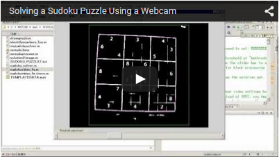
There is a fun video that shows you how you can solve Sudoku puzzles using a webcam that uses a different character recognition technique. Instead of static images, our colleague Teja Muppirala uses a live video feed in real time to do it and he walks you through the pre-processing steps one by one. You should definitely check it out: Solving a Sudoku Puzzle Using a Webcam.
Submitting Your Entry to Kaggle
You got 96% categorization accuracy rate by simply accepting the default settings except for the number of hidden neurons. Not bad for the first try. Since you are using a Kaggle dataset, you can now submit your result to Kaggle.
n = size(sub, 1);                                   % num of samples
sub = sub';                                         % transpose
[~, highest] = max(scores);                         % highest scoring model
net = models{highest};                              % restore the model
Ypred = net(sub);                                   % label probabilities
[~, Label] = max(Ypred);                            % predicted labels
Label = Label';                                     % transpose Label
Label(Label == 10) = 0;                             % change '10' to '0'
ImageId = 1:n; ImageId = ImageId';                  % image ids
writetable(table(ImageId, Label), 'submission.csv');% write to csv
You can now submit the submission.csv on Kaggle's entry submission page.
Closing
In this example we focused on getting a high level intuition on artificial neural network using a concrete example of handwritten digit recognition. We didn’t go into details such as how the inputs weights and bias units are combined, how activation works, how you train such a network, etc. But you now know enough to use Deep Learning Toolbox in MATLAB to participate in a Kaggle competition.
- 범주:
- Machine learning


댓글
댓글을 남기려면 링크 를 클릭하여 MathWorks 계정에 로그인하거나 계정을 새로 만드십시오.