
The Perverse Port Passing Problem
Today's guest blogger is Jos Martin, from the Parallel Computing group at MathWorks. Whilst normally focussing on making parallel computing both easy and fast in MATLAB, occasionally he likes to use MATLAB to explore other problem spaces. Here, he writes about an interesting random walk process he encountered that has allowed him to explore both simulation and analytic methods in MATLAB, and using each of those methods to help guide the other.
 From this histogram we feel greatly relieved! It shows that no matter where we sit at the table, the number of times we are the last person to receive the port is the same as everyone else. It does not matter where we sit at the table!
This result seems somewhat counter intuitive; surely how far you are from the starting position should affect the likelihood you are last? First let's see if this result is the same for a different table size. We can check by running the simulator with a larger number of people.
From this histogram we feel greatly relieved! It shows that no matter where we sit at the table, the number of times we are the last person to receive the port is the same as everyone else. It does not matter where we sit at the table!
This result seems somewhat counter intuitive; surely how far you are from the starting position should affect the likelihood you are last? First let's see if this result is the same for a different table size. We can check by running the simulator with a larger number of people.
 There is an intuitive way to describe that the probability of being last is independent of where you sit at the table. To be last, the decanter must have arrived at your left or right, then traversed the whole table without passing via you. No matter where you sit at the table, the probability of that set of actions is the same - and thus the probability of you being last is the same.
In terms of $pSAB$ this can be written as:
There is an intuitive way to describe that the probability of being last is independent of where you sit at the table. To be last, the decanter must have arrived at your left or right, then traversed the whole table without passing via you. No matter where you sit at the table, the probability of that set of actions is the same - and thus the probability of you being last is the same.
In terms of $pSAB$ this can be written as:
 It is clear from this histogram that even a small bias in the probability hugely affects the likelihood we will be last. We could undertake studies to decide how many dinner parties we needed to attend before we could reasonably deduce that the decanter was biased, but that is another story!
 From the graph we can see that guests who are close to the initial position of the decanter (location 1) receive and pass the port a little less than twice as often (for this size table) as the guest opposite them, and that as the passing becomes biased so one side of the table is more likely to receive more wine than the other side. We can also see that the unbiased case has the largest number of passes on average, which we can guess by considering that in the case p==1 (or p==0) the number of times each location receives the port is just once!
 There looks to be a quadratic relationship here; the interested reader is encouraged to explore this and produce a functional form for the relationship as table size changes and to look at how the average number of visits scales as the table size increases.
 If you are interested, it is worth looking at this distribution using Distribution Fitter from the Statistics and Machine Learning Toolbox. It seems to be well fitted using either Lognormal or Birnbaum-Saunders distributions. We can fit either of these using the fitdist function and plot the expected distribution over the histogram
 We can use a probability plot to see how well the LogNormal distribution fits the data. You can see that in the tails the distribution is incorrect.
 Both LogNormal and Birnbaum-Sanders over-estimate the number of passes around the mean and underestimate around 1.5 times the mean, so whilst fitting fairly well they don't actually model the distribution correctly. The mean of the fitted and actual distributions is shown below.
 It looks like there is a very strong polynomial relationship between these quantities. What does a polynomial fit of degree 4 and degree 2 look like?
 Finally, we could test the likelihood that the data was drawn from that fitted distribution, but with zero mean, using a chi-squared goodness of fit test
 Finally, looking at what happens if the situation becomes biased, we probably expect that the position with the longest expected path will shift to one side (i.e. closer to the start position). In fact, thinking about the limit where p approaches 1 we should expect that the path length to position N-1 simply becomes N (since the decanter will pass from k to k+1 with probability close to 1). The path length for N-2 will probably be very close to that for N-1, with a deviation to the right somewhere around the table (with close to zero probability). Thus for p > 0.5 we expect the peak in the path length to move towards position zero and for the expected path length for k = N-1 to be shorter than for k = 1.
Contents
- Introduction
- A simulation approach
- Investigating the final position of the port
- Analytic probability for last position when passing is unbiased
- What happens if there is a biased probability of passing left or right?
- Does this biased simulation agree with theory?
- Who has the most to drink?
- Does the number of guests affect how much each drinks?
- Will the pipe of port run out?
- Predicting the amount of port consumed
- An analytic conjecture
- How does the amount of port consumed depend on the final position?
- And finally
Introduction
Pi day is coming and you have been invited to dine with an eccentric but mathematically minded host. She has provided many interesting delicacies and you have now finally arrived at the cheese course; of course port is served alongside a wonderful round of Stilton. However, in defiance of normal protocol (passing to the left), she instructs her guests to randomly choose a direction in which to pass the port decanter. You are some way around the circular table and feeling a degree of consternation at this strange turn of events. Should you be concerned? How does your position at the table affect the likelihood of being the last person to sample this exceptional Fonseca '63? For those pedantic few who immediately worry that the port might run out, I can assert she is a very accommodating host and has assured her guests that the decanter will continue to be filled from the pipe of port she recently acquired. Another question one might pose is: on average how much port will be consumed (assuming that at each pass each guest takes a fixed amount of port)? This problem can be modelled with a random walk, similar in nature to a well-studied case called Gambler's Ruin. The major difference here will be the need to visit all locations around the table, rather than simply reaching one end or other of the walk. To explore this apparently simple problem I will start by using a simulation approach that will help guide analytic methods (in a future post). To do this I'll be using our statistics and symbolic maths tools.A simulation approach
There are analytical methods to attack this problem (I will quote some of these during this article, for which all files and proofs are available on File Exchange) but here I want to focus on a monte-carlo simulation approach. To exemplify the approach, we will run nSims independent simulations passing the decanter between N people (always starting at person 0), with a probability p of passing left (and 1-p of passing right).nSims = 100; N = 11; p = 0.5;To simulate M passes of the port across the nSims simulations we make a matrix singleMove containing only values 1 and -1 to indicate a pass to the port to left or right using uniform random numbers.
M = 25;
singleMove = 2*(rand(nSims, M) >= p) - 1;
% The first 6 pass directions of 6 simulations
disp(singleMove(1:6, 1:6));
    -1    -1     1     1     1    -1
    -1    -1     1     1    -1     1
    -1     1    -1     1    -1    -1
    -1     1     1     1    -1    -1
    -1     1    -1     1     1    -1
    -1    -1    -1    -1     1     1
By knowing the direction of each pass we can compute the location of the port compared to its starting point by taking the cumulative sum of the directions for each pass. To make this an absolute position we add to it the starting position (in this case position 0). Because we need to account for the decanter moving all the way around the table, we are going to use modulo N arithmetic to fold the course back to the available positions.
start = 0;
locations = mod(cumsum(singleMove, 2) + start, N);
% The first 6 locations of 6 simulations
disp(locations(1:6, 1:6))
    10     9    10     0     1     0
    10     9    10     0    10     0
    10     0    10     0    10     9
    10     0     1     2     1     0
    10     0    10     0     1     0
    10     9     8     7     8     9
We now have a matrix locations that contains 100 simulations of 20 passes. Have any of the simulations reached all places around the table? In the function portPassingSimulation we are going to iterate over each pass seeing which simulations complete in that pass, but here we will simply work out if any of the simulations are complete. To be complete, a simulation needs to have visited all 0:N-1 possible locations. A simple way to ask this question is to see if that simulation contains N unique elements. If it does, it must have visited all the possible locations.
finished = false(nSims, 1);
for ii = 1:nSims
    finished(ii) = numel(unique(locations(ii, :))) == N;
end
nFinished = sum(finished)
nFinished =
    10
For those simulations that have not finished, we know their current location (given by locations(:,end)) and so can simulate another block of nSims x M passes, keeping on going until all simulations have reached their goal. The full simulation code (portPassingSimulation available here) returns the last position, the number of passes to reach that position, the direction the last position was reached and the number of visits to each position around the table during each simulation. The code is based closely on this strategy, with a slightly different stopping detection strategy.
[last, nPasses] = portPassingSimulation(nSims, N, p);
results = table(last, nPasses);
disp(results(1:10,:))
    last    nPasses
    ____    _______
     7      215
     7      129
     8      127
     8      127
     3      124
    10      108
     4      102
     8      102
     5      101
     3       98
Investigating the final position of the port
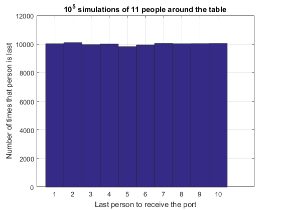
The first problem we set ourselves was deciding if our position around the table affected our probability of being the last person to receive the port. To look at this, let's run a fairly large number ($10^5$) of simulations and see how many end up at each of the N-1 possible finishing positions.last = portPassingSimulation(1e5, N, p); hist(last, 1:N-1); grid on title '10^5 simulations of 11 people around the table' xlabel 'Last person to receive the port' ylabel 'Number of times that person is last'
From this histogram we feel greatly relieved! It shows that no matter where we sit at the table, the number of times we are the last person to receive the port is the same as everyone else. It does not matter where we sit at the table!
This result seems somewhat counter intuitive; surely how far you are from the starting position should affect the likelihood you are last? First let's see if this result is the same for a different table size. We can check by running the simulator with a larger number of people.
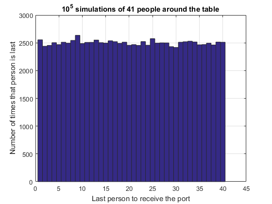
last = portPassingSimulation(1e5, 41, p);
hist(last, 1:max(last));
grid on
title '10^5 simulations of 41 people around the table'
xlabel 'Last person to receive the port'
ylabel 'Number of times that person is last'
There is an intuitive way to describe that the probability of being last is independent of where you sit at the table. To be last, the decanter must have arrived at your left or right, then traversed the whole table without passing via you. No matter where you sit at the table, the probability of that set of actions is the same - and thus the probability of you being last is the same.
Analytic probability for last position when passing is unbiased
We can show analytically that the likelihood of being last is independent of your position around the table. We will need to quote a result from the Gamblers Ruin analysis. Let $pSAB$ be the probability that the decanter starts at position S and reaches position A before reaching position B. This probability is identical to starting with an initial stake of (S-B) in Gambler's Ruin and stopping when either the stake is lost or the winnings are (A-B). $$pSAB=\frac{S-B}{A-B}\mbox{ for }B<S<A\mbox{ or }A<S<B$$ We can use the Symbolic Math Toolbox to manipulate equations without having to do the algebra ourselves (for me, making a transcription mistake much less likely). In this case the probability that some position k is the last is a combination of- Starting at position 0 and going to position L (numbered k-1) whilst not going to position R (numbered k+1), followed by going from position L to position R whilst not going to position k
- Starting at position 0 and going to position R whilst not going to position L, followed by going from position R to position L whilst not going to position k
syms pSAB(S,A,B) k N
pSAB(S,A,B) = (S-B)/(A-B);
L = k-1;
R = k+1-N;
pLastUnbiased = simplify(pSAB(0,L,R)*pSAB(L,R,k) + pSAB(0,R,L)*pSAB(R,L,k-N))
pLastUnbiased =
1/(N - 1)
Note that to ensure that either $A<S<B \mbox{ or } B<S<A$ we sometimes need to undertake a modulo approach to A or B. That is why R is written k+1-N and why in the last term we use k-N rather than just k. This ensures that $k>L \ge 0 \ge R > k-N$. The result pLast is independent of k and shows equal likelihood of being last, agreeing with the simulation.
What happens if there is a biased probability of passing left or right?
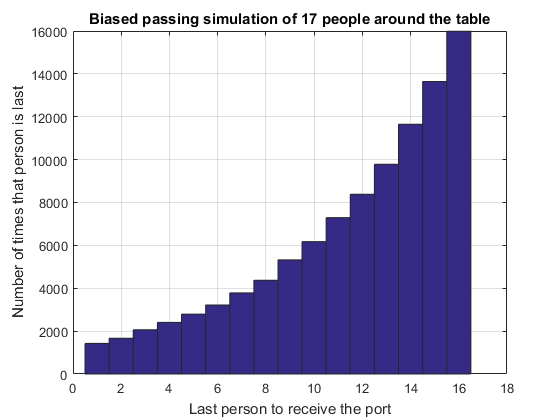
The above simulations have assumed that the probability that any dinner guest passes left or right are equal. What if there is a slight bias to one direction? Will this have a discernible impact on your enjoyment of the port? Let's simulate a situation where the probability of passing left is 0.54 (rather than 0.5).N = 17; p = 0.54; k = 1:N-1; nSims = 1e5; last = portPassingSimulation(nSims, N, p); hist(last, k); grid on title 'Biased passing simulation of 17 people around the table' xlabel 'Last person to receive the port' ylabel 'Number of times that person is last'
It is clear from this histogram that even a small bias in the probability hugely affects the likelihood we will be last. We could undertake studies to decide how many dinner parties we needed to attend before we could reasonably deduce that the decanter was biased, but that is another story!
Does this biased simulation agree with theory?
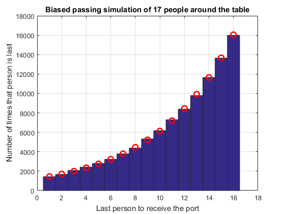
Using a very similar approach to the analytic method above (see the next post (not live right away) for a derivation) we can show that the biased probability of being last is $$P_{last}=\frac{r^N(1-r)}{r^k(r-r^N)} \mbox{ where }r=\frac{1-p}{p} \mbox{ and } p\ne \frac{1}{2}$$ Plotting that on top of the simulation shows very good agreement.r = (1-p)/p; pLastBiased = r^N*(1-r)./(r.^k*(r-r^N)); hold on plot(k, pLastBiased*nSims, 'ro', 'MarkerSize', 8, 'LineWidth', 2); hold off
Who has the most to drink?
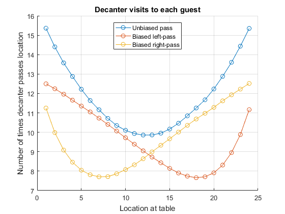
Now that we know each guest is equally likely to be the last to receive the port, we could look at the total number of times that the decanter passes each guest on its travels to the last person. Is this the same for each person around the table or not? And does having a biased passing probability change the number of times it passes each person?nSims = 3e4; N = 25; [~, ~, ~, visitsUnbiased] = portPassingSimulation(nSims, N, 0.5); [~, ~, ~, visitsBiasedL] = portPassingSimulation(nSims, N, 0.53); [~, ~, ~, visitsBiasedR] = portPassingSimulation(nSims, N, 0.47); figure hold on plot(1:N-1, visitsUnbiased/nSims, 'o-') plot(1:N-1, visitsBiasedL/nSims, 'o-') plot(1:N-1, visitsBiasedR/nSims, 'o-') hold off grid on legend('Unbiased pass', 'Biased left-pass', 'Biased right-pass', 'Location', 'N') title 'Decanter visits to each guest' xlabel 'Location at table' ylabel 'Number of times decanter passes location'
From the graph we can see that guests who are close to the initial position of the decanter (location 1) receive and pass the port a little less than twice as often (for this size table) as the guest opposite them, and that as the passing becomes biased so one side of the table is more likely to receive more wine than the other side. We can also see that the unbiased case has the largest number of passes on average, which we can guess by considering that in the case p==1 (or p==0) the number of times each location receives the port is just once!
Does the number of guests affect how much each drinks?
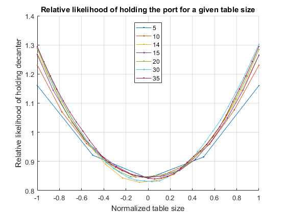
The above graph was for a single table size (N == 25). What happens if we have different table sizes? Is there a fundamental relationship between how many visits the port makes to each location? Clearly we are going to need a way to compare the visits at different sized tables and with different numbers of simulations. We will plot all results for a normalized location [-1 1] which maps to our integer locations 1:N-1. In addition, we need to normalize the visits in some way. To do this we will scale the number of visits to each location as a proportion of the number expected for that table if each location were passed equally. To do this we divide the number of visits to each location by the total number of visits and multiply by the number of people at the table. For a table that had each location equally attended, this would produce the value 1 at each location, indicating that the expected number of visits to that location is 1 times the equally distributed number.figure hold on grid on tableSizes = [5 10 14 15 20 30 35]; for kk = tableSizes [~, ~, ~, visits] = portPassingSimulation(1e4, kk+1, 0.5); plot( linspace(-1, 1, kk), kk*visits/sum(visits), '.-') end hold off legend(string(tableSizes), 'Location', 'N') title 'Relative likelihood of holding the port for a given table size' xlabel 'Normalized table size' ylabel 'Relative likelihood of holding decanter'
There looks to be a quadratic relationship here; the interested reader is encouraged to explore this and produce a functional form for the relationship as table size changes and to look at how the average number of visits scales as the table size increases.
Will the pipe of port run out?
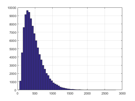
Let's assume that each of the guests takes 2 fl.oz. (a shot) of port every time the decanter passes them. We can then calculate how much port is consumed in a given simulation by tracking the number of iterations each simulation took to finish. The second output of portPassingSimulation returns the number of passes needed to reach the final location. Across all simulations this will give us a distribution function for passes needed to finish.nSims = 1e5; N = 31; p = 0.5; binW = 50; [~, nPasses] = portPassingSimulation(nSims, N, p); hist(nPasses, 30:binW:max(nPasses)); hold on grid on
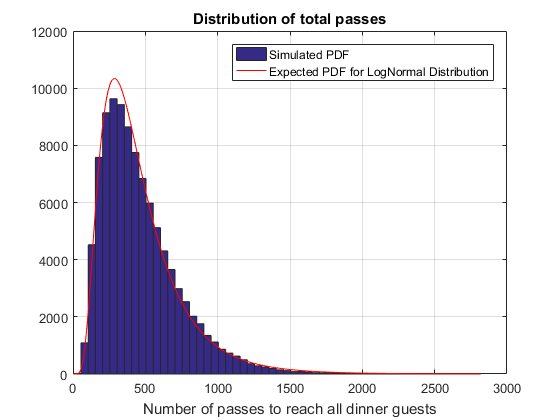
If you are interested, it is worth looking at this distribution using Distribution Fitter from the Statistics and Machine Learning Toolbox. It seems to be well fitted using either Lognormal or Birnbaum-Saunders distributions. We can fit either of these using the fitdist function and plot the expected distribution over the histogram
pd = fitdist(nPasses, 'LogNormal')
x = linspace(1, max(nPasses), 200);
plot(x, nSims*binW*pdf(pd, x), 'r');
hold off
title 'Distribution of total passes'
xlabel 'Number of passes to reach all dinner guests'
legend('Simulated PDF', 'Expected PDF for LogNormal Distribution')
pd =
  LognormalDistribution

  Lognormal distribution
       mu =  5.98543   [5.98189, 5.98897]
    sigma = 0.570894   [0.568403, 0.573407]
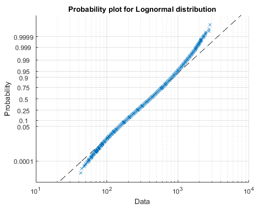
We can use a probability plot to see how well the LogNormal distribution fits the data. You can see that in the tails the distribution is incorrect.
probplot('LogNormal', nPasses)
grid on
Both LogNormal and Birnbaum-Sanders over-estimate the number of passes around the mean and underestimate around 1.5 times the mean, so whilst fitting fairly well they don't actually model the distribution correctly. The mean of the fitted and actual distributions is shown below.
fittedMean = pd.mean
actualMean = mean(nPasses)
fittedMean =
       467.96
actualMean =
       465.29
To account for this inability to fit the simulation data we are going to use the empirical mean for the rest of this analysis. If we were more sure that we understood the expected distribution, we would use a fitted distribution.
Predicting the amount of port consumed
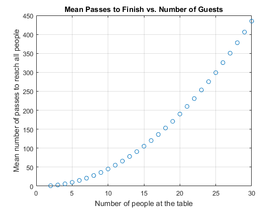
Next let's investigate if there is a simple relationship between the number of people at the table and the expected number of passes for the port to go around the table. We can do this by running a number of different simulations, looking at the relationship between the mean and number of people. Let's do this for dinner tables of size 2:30 with unbiased passing probability. To speed up the computation we use a parallel for-loop from the Parallel Computing Toolbox, since each of the simulations is independent of the others. By default, this will automatically open a parallel pool if one isn't already open.p = 0.5; tableSize = 2:30; tToFinish = zeros(size(tableSize)); parfor ii = 1:numel(tableSize) [~, nPasses] = portPassingSimulation(1e5, tableSize(ii), p); tToFinish(ii) = mean(nPasses); end plot(tableSize, tToFinish, 'o') title 'Mean Passes to Finish vs. Number of Guests' xlabel 'Number of people at the table' ylabel 'Mean number of passes to reach all people' grid on
It looks like there is a very strong polynomial relationship between these quantities. What does a polynomial fit of degree 4 and degree 2 look like?
f4 = polyfit(tableSize, tToFinish, 4)
f2 = polyfit(tableSize, tToFinish, 2)
f4 =
   1.8679e-05   -0.0011103      0.52081     -0.63573      0.24387
f2 =
      0.49955     -0.49157    -0.015421
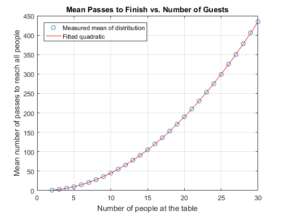
Notice how the 3rd and 4th order parameters of f4 are basically zero? This shows that the data is well fitted using just a second-order polynomial.
hold on
x = linspace(min(tableSize), max(tableSize), 100);
plot(x, polyval(f2, x), 'r');
hold off
legend('Measured mean of distribution', 'Fitted quadratic', 'Location', 'NW')
An analytic conjecture
Also I noticed how close the values of f2 are to [0.5 -0.5 0]. This seems too good to be true! If you run more simulations (for example with tables sizes from 2:100) with a larger number of simulations per table size, the polynomial fit to the mean gets closer to this set of values. My conjecture is that for a table of size N $$E(\mbox{passes to finish}) = \frac{N(N-1)}{2}$$ We can try out this conjecture for a few table sizes by running a number of different simulations, taking away the expected number of passes for that table size and looking at the residuals to see if their mean is zero.residuals = zeros(60,1); parfor ii = 1:60 % Use table sizes 9:4:29 N = 9 + 4*mod(ii, 6); [~, nPasses] = portPassingSimulation(1e5, N, 0.5); eMeanPasses = polyval([0.5 -0.5 0], N); residuals(ii) = mean(nPasses) - eMeanPasses; end % Are the residuals drawn from a normal distribution with zero mean? We can % use a t-test to look at this [H1, pVal1, CI, stats] = ttest(residuals)
H1 =
     0
pVal1 =
      0.32436
CI =
     -0.18322
     0.061617
stats =
  struct with fields:

    tstat: -0.99384
       df: 59
       sd: 0.47389
The output (H==0) from t-test shows that we cannot reject the null hypothesis - the data could be drawn from a normal distribution with zero mean, and with only with probability pVal would we expect a distribution less like a normal one be drawn at random.
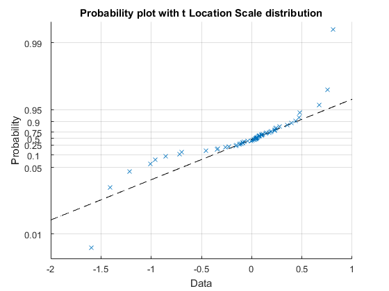
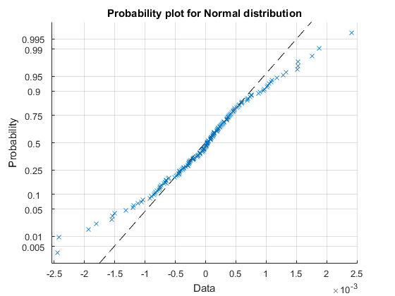
Looking at a number of these results we can see that the tails of the distribution are not actually normal, so we can use a "t-location scale" probability plot to see how well the residuals are fitted by the distribution. If it fits well then all the points should be on the straight line.
pd = fitdist(residuals, 'tLocationScale');
probplot(pd, residuals)
grid on
title 'Probability plot with t Location Scale distribution'
Finally, we could test the likelihood that the data was drawn from that fitted distribution, but with zero mean, using a chi-squared goodness of fit test
pd.mu = 0;
[H2, pVal2] = chi2gof(residuals, 'cdf', pd)
H2 =
     0
pVal2 =
      0.57262
That seems to fit reasonably well, indicating that our conjecture seems to fit the data. See my next blog post for an analytic proof of this conjecture. So we can now finally answer the question about the pipe of port running out, since we can predict the mean number of passes for a given table size.
% 1008 Imperial Pints in a Pipe and 2 fl.oz. glass
% and 20 fl.oz. in Imperial Pint
pintsInPipeOfPort = 1008;
maxPasses = pintsInPipeOfPort*20/2;
N = sym('N');
assume(N > 0)
% Use the Symbolic Math Toolbox to solve the equation for k
double(solve( N*(N-1)/2 == maxPasses, N ))
ans =
       142.49
This tells us that with a table size of 142 less than half of her dinners will run out of port!
How does the amount of port consumed depend on the final position?
One final aspect of the problem that we can investigate is how the overall path length (and hence amount of port consumed) varies depending on the position that comes last. Thinking about the paths that need to be taken for positions near the starting point to be last as opposed to ones further away we might intuitively think that the nearer ones might be shorter. Let's see if this is the case, and how the paths change as the passing becomes biased. Firstly, we need to run the simulation (unbiased for a table of size 17).N = 17; p = 0.5; [last, nPasses] = portPassingSimulation(5e5, N, p);Next, look at the mean of the number of passes, but group those means by the possible last position. There is a really easy way to do this using the varfun method of a table, and grouping by the variable last.
G = varfun(@mean, table(last, nPasses), 'GroupingVariable', 'last')
G =
    last    GroupCount    mean_nPasses
    ____    __________    ____________
     1      31392         100.71
     2      31392         114.98
     3      31256         127.18
     4      31205          137.1
     5      31209         144.15
     6      31254         151.21
     7      31255         155.31
     8      31429         156.65
     9      30950         156.79
    10      31405         155.29
    11      31182         150.78
    12      31333         144.77
    13      31276         136.87
    14      31015          127.2
    15      31313         115.35
    16      31134         100.88
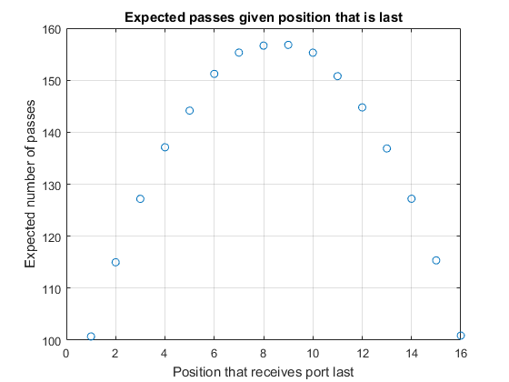
Plotting the mean passes we can see that positions closest to zero have the shortest paths and those furthest away the longest.
plot(G.last, G.mean_nPasses, 'o')
title  'Expected passes given position that is last'
xlabel 'Position that receives port last'
ylabel 'Expected number of passes'
grid on
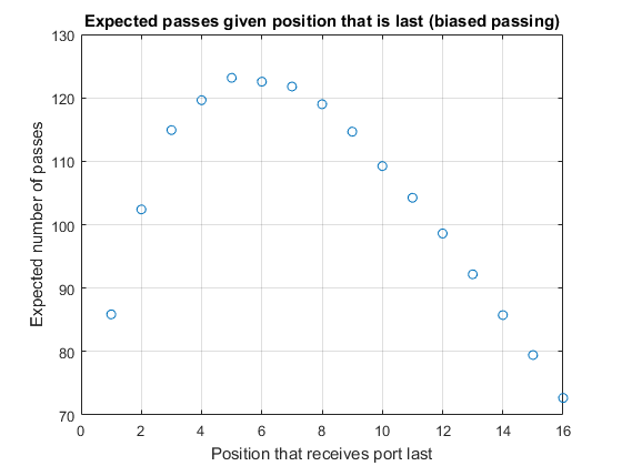
Finally, looking at what happens if the situation becomes biased, we probably expect that the position with the longest expected path will shift to one side (i.e. closer to the start position). In fact, thinking about the limit where p approaches 1 we should expect that the path length to position N-1 simply becomes N (since the decanter will pass from k to k+1 with probability close to 1). The path length for N-2 will probably be very close to that for N-1, with a deviation to the right somewhere around the table (with close to zero probability). Thus for p > 0.5 we expect the peak in the path length to move towards position zero and for the expected path length for k = N-1 to be shorter than for k = 1.
N = 17;
p = 0.57;
[last, nPasses] = portPassingSimulation(5e5, N, p);
G = varfun(@mean, table(last, nPasses), 'GroupingVariable', 'last');
plot(G.last, G.mean_nPasses, 'o')
title  'Expected passes given position that is last (biased passing)'
xlabel 'Position that receives port last'
ylabel 'Expected number of passes'
grid on


Comments
To leave a comment, please click here to sign in to your MathWorks Account or create a new one.