Jiro's pick this week is multicomet by Ben.

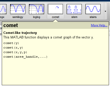
Did you know that we had a function called comet that allows you to animate trajectory plots? It was like a hidden gem for me when I found it. It's a simple concept, but very useful for when I wanted to animate my signal trace. There was no need for me to write loops to update my graphics. With the new toolstrip, you can find it right away.

Ben extended comet to work with multiple trajectories. Now it's easy to visualize multi-state dynamics, such as the Lotka-Volterra predator-prey model.

$$y_1' = (1 - \alpha \cdot y_2) \cdot y_1$$

$$y_2' = (-1 + \beta \cdot y_1) \cdot y_2$$

The prey population increases when there are no predators, and the predator population decreases when there are no prey. Let's use the example function lotka that uses $\alpha = 0.01$ and $\beta = 0.02$.

type lotka

function yp = lotka(t,y)
%LOTKA  Lotka-Volterra predator-prey model.

%   Copyright 1984-2002 The MathWorks, Inc. 
%   $Revision: 5.7 $  $Date: 2002/04/15 03:33:21 $

yp = diag([1 - .01*y(2), -1 + .02*y(1)])*y;

% Define initial conditions.
y0 = [20; 20];

% Simulate the differential equation.
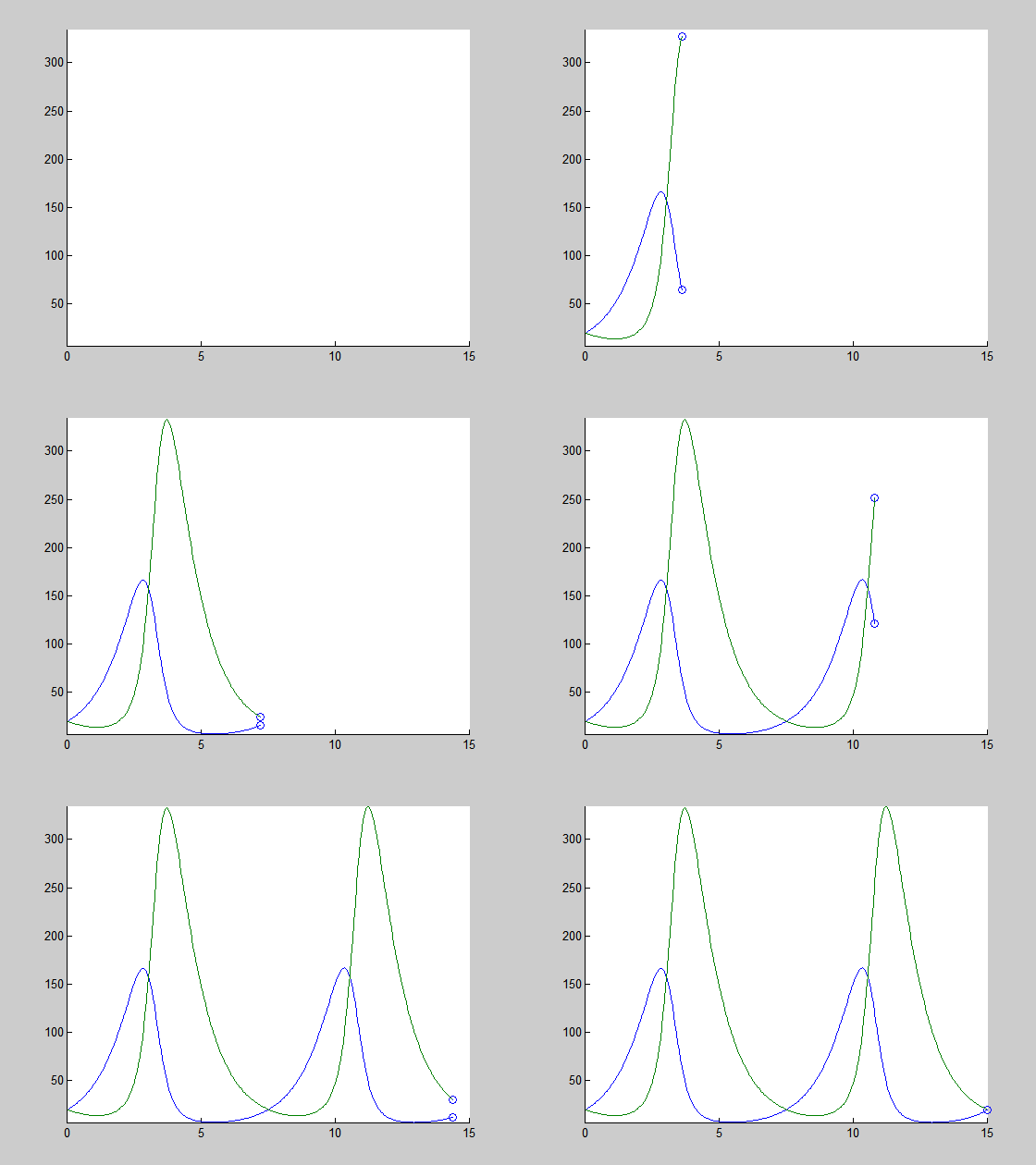
[t,y] = ode45(@lotka, 0:0.005:15, y0);

% Animate.
multicomet(t, y)

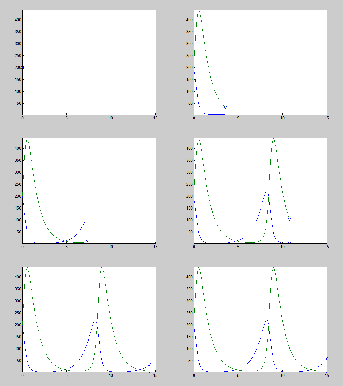
Let's try different initial conditions.

y0 = [200; 200];

[t,y] = ode45(@lotka, 0:0.005:15, y0);

multicomet(t, y)

Thanks, Ben, for this nice extension to comet!

Comments

What are some of your favorite way of animating your data? Tell us about it here.

Get the MATLAB code

Published with MATLAB® R2013a

Published with MATLAB® R2013a