
Divergent colormaps
I promised earlier to post about divergent colormaps. A divergent colormap is usually constructed by concatenating two colormaps together that have different color schemes.
Here is an example of a divergent colormap from www.ColorBrewer.org by Cynthia A. Brewer, Geography, Pennsylvania State University.
rgb = [ ...
    94    79   162
    50   136   189
   102   194   165
   171   221   164
   230   245   152
   255   255   191
   254   224   139
   253   174    97
   244   109    67
   213    62    79
   158     1    66  ] / 255;

b = repmat(linspace(0,1,200),20,1);
imshow(b,[],'InitialMagnification','fit')
colormap(rgb)
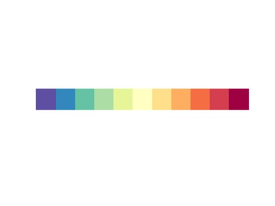
This colormap has the brightest color in this middle, which is typical for divergent colormaps.
A divergent colormap is used to compare data values to a reference value in a way that visually highlights whether values are above or below the reference.
Let me show you an example using sea surface temperatures. I learned today that 28 degrees Celsius has a specific meaning in hurricane modeling and prediction. It is considered to be the minimum temperature for hurricane formation.
Using the NASA EOSDIS Reverb tool, I found and downloaded sea surface temperature from the Aqua satellite for August 1, 2011. The data arrived as a netCDF file.
amsre = ncread('20110801-AMSRE-REMSS-L2P_GRIDDED_25-amsre_20110801rt-v01.nc',...
    'sea_surface_temperature');

size(amsre)
ans =

        1440         720           2
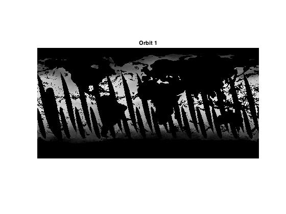
The two planes contain data from two different orbits.
orbit1 = flipud(amsre(:,:,1)');
orbit2 = flipud(amsre(:,:,2)');

imshow(orbit1,[],'InitialMagnification','fit')
title('Orbit 1')
imshow(orbit2,[],'InitialMagnification','fit')
title('Orbit 2')
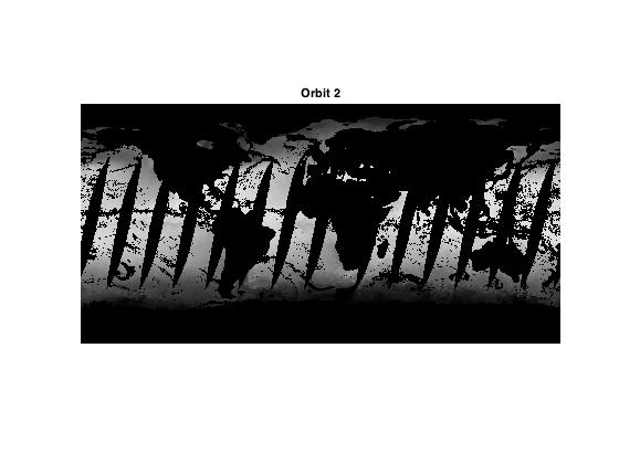
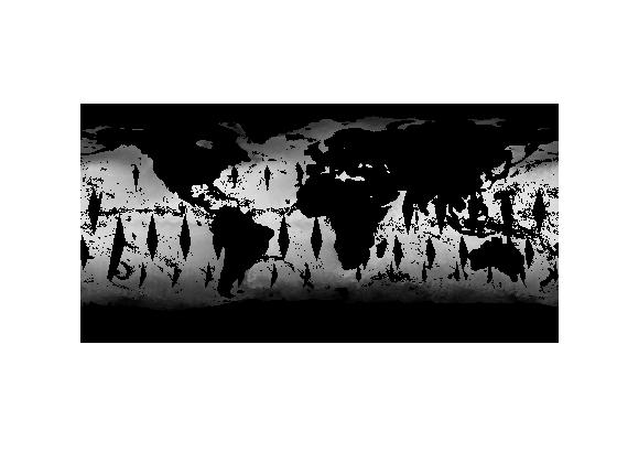
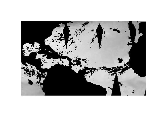
The black regions are NaNs representing missing data. Combine the two orbits by taking the maximum.
sst = max(orbit1,orbit2);
imshow(sst,[],'InitialMagnification','fit')
Now grab a subset of the data that includes a portion of the Atlantic Ocean.
ssta = sst(180:400,330:700);
imshow(ssta,[],'InitialMagnification','fit')
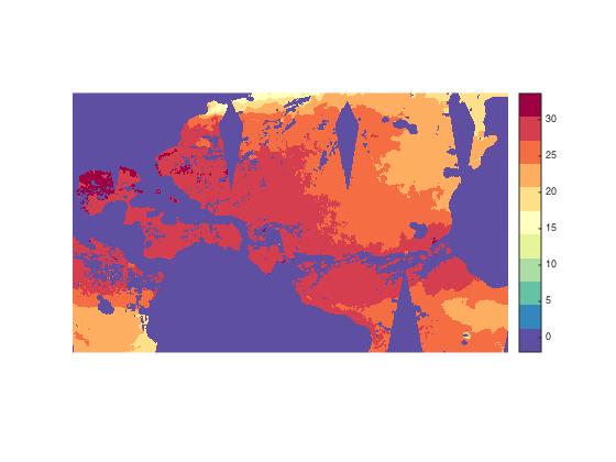
Apply the divergent colormap.
colormap(rgb)
colorbar

OK, I see one problem right off the bat. It looks like our data is in Kelvin. Let's fix that.
ssta = ssta - 273.15;
imshow(ssta,[],'InitialMagnification','fit')
colormap(rgb)
colorbar
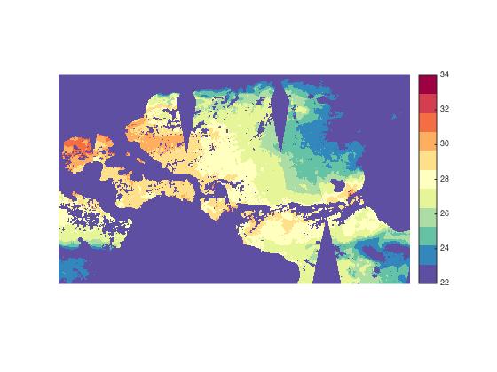
Now I want to make use of our divergent colormap to highlight the temperature of interest, 28 degrees. To do that, I'll use the CLim property of the axes object. The CLim property is a two-element vector. The first element tells us the data value that maps to the lowest colormap color, and the second element tells us the data value that maps to the highest colormap color. MATLAB computes these values automatically based on the range of the data.
get(gca,'CLim')
ans =

   -1.9500   33.6000
To get the middle colormap color to represent 28 degrees, we need to pick our two CLim values so that they are equally far away from 28 degrees. After some experimentation, I settled on a range from 22 degrees to 34 degrees.
set(gca,'CLim',[22 34])
That's looking better, but it isn't helpful to have the missing data displayed using the bottom color of the colormap. I will fix that problem using this procedure.
- Construct a gray mask image (in truecolor format).
- Display it on top of our sea surface temperature image.
- Set the AlphaData of the gray mask image so that the sea surface temperatures show through.
Here are just the first two steps.
mask = isnan(ssta);
graymask = 0.5 * mask;
graymask = repmat(graymask,1,1,3);
hold on
h = imshow(graymask);
hold off
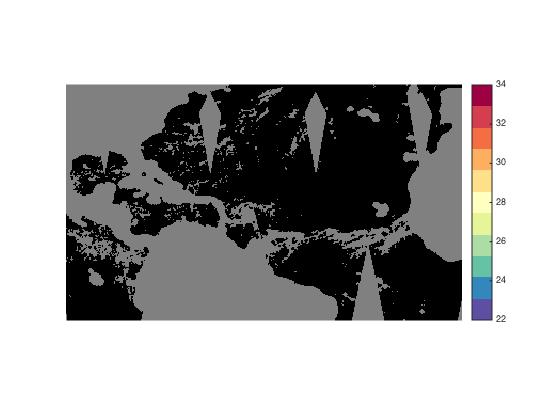
The missing values are displayed as gray, but we can't see the sea surface temperatures. Fix that by using the NaN-mask as the overlay image's AlphaData.
h.AlphaData = mask; % This syntax requires MATLAB R2014b.
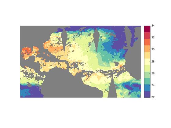
Temperatures close to the threshold are displayed using yellow, the brightest color in the colormap and the one right in the middle. Temperatures above the threshold are displayed using oranges and reds, while temperatures below are displayed using greens and blues.
Before I go, I want to give a shout to the new Developer Zone blog that just started today. If you are into advanced software developer topics, I encourage you to head over there and take a look.
- Category:
- Colormap


Comments
To leave a comment, please click here to sign in to your MathWorks Account or create a new one.