
Magic Formula Tire Modeling in Formula Student
For today’s blog post, Veer Alakshendra is happy to host Tom Teasdale from the UPBracing Formula Student team. Tom is here to discuss about the tool that he has developed for tire modeling.
Introduction
This blog post will briefly introduce Magic Formula Tire and a new, open-source MATLAB tool for creating, fitting, and evaluating Magic Formula Tire models. It is tailored for students trying to implement tire models using data from the FSAE Tire Test Consortium (FSAE TTC). You can export your fitted model as a TIR-file or as a struct to use outside of this tool.
Motivation
Are you a student participating in the Formula Student (FSAE) competition? If your answer is yes, you know how heavily your car is influenced by your tires. Limiting the maximum transmissible force of your engine (or motors) to the road, tire characteristics should be understood and compared to make a qualified tire choice. You might also be developing a Vehicle Dynamics Control algorithm or a high-fidelity vehicle model in MATLAB/Simulink for which you also need a model representation of your car’s tire. As an active student in Formula Student myself, those were the typical challenges we had to face at my team UPBracing.
Luckily, Formula Student teams can gain access to high-quality tire data by becoming members of the FSAE Tire Test Consortium. For a small membership fee, you can download complete data of most Formula Student tires which we can then use to create highly accurate and computationally efficient, empirical tire models.
Magic Formula Tire is not the only empirical tire modeling approach out there. It is only one of many. However, it is also the most popular one (neglecting the linear tire model), and for good reasons. It can be understood as an advanced version of the famous, classic Magic Formula.
$ y = D \cdot \sin \bigg( C \cdot \arctan \Big( B \cdot x – E\big( B \cdot x – \arctan(B \cdot x) \big) \Big) \bigg) $
where y is the output variable (e.g. lateral tyre force) and x the input variable (e.g. slip angle). B, C,D and E are the tuning parameters.
For an example of how you can fit the classic Magic Formula to data, you can refer to Analyzing Tire Test Data, a blog post by MathWorks staff. In their case, the fitting results in a large interpolation grid which alters the parameters depending on the current steady-state conditions. But interpolation grids can be disadvantageous, especially where execution speed matters and they are also hard to modify after the fitting process.
A more advanced version of the classical Magic Formula is the semi-empirical Magic Formula model with around 100 parameters. Semi-empirical means that the model incorporates knowledge about tire dynamics in its equations and is not purely empirical as, for example, a polynomial model. Therefore, semi-empirical Magic Formula models can also realistically extrapolate tire characteristics using the so-called similarity method. This is very useful, as we usually don’t have test-bench data for every possible steady-state. The TTC for example only tests slip angles up to about 6 degrees. Although the model seems really complex with over 100 parameters to tune, we usually only need a fraction of those for a great model-data-fit. But, to be fair, it can be a bit cumbersome to build Magic Formula Tire models with just MATLAB scripts, especially if you want to manually tune parameters. I hope that my tool can help students in that regard.
In the following, any reference to Magic Formula or Magic Formula Tire implies its semi-empirical form.
Methodology
The Magic Formula Tire Tool showcased here can be understood as an open-source alternative to multiple commercial solution to fitting Magic Formula Tire models to data. It acts as a graphical wrapper to the closely related project Magic Formula Tire MATLAB Library, which is a collection of command-line tools. This means, that almost everything done by the GUI can be done with just the library in the MATLAB console. It also means that the Magic Formula Tire equations used in the GUI for fitting are the same as in the library. So the fitted parameter set yields the same results in the GUI as with the Command-Line tools in the Magic Formula Tire MATLAB Library.
By the way, the evaluation functions in the library mentioned above are code-generation compatible and have been used for that purpose at UPBracing. So feel free to fit your model using the GUI and evaluate it using the library in your code-generation projects.
Implementing Magic Formula Tire
For those who want to understand the implementation of Magic Formula Tire model, I will provide a short summary. Here the definitive reference is the book Tire and Vehicle Dynamics by Hans B. Pacejka (2012). In chapter 4.3.2. you will find the full set of equations. You should also keep the MF-Tyre/MF-Swift manual nearby as a sort of cheatsheet for the parameters. Implementing these is pretty straightforward. Let’s take a peak at the source-code for Fx0, which calculates longitudinal tire force for pure longitudinal slip.
function [Fx0,mux,Cx,Dx,Ex] = Fx0(p,longslip,inclangl,pressure,Fz)
% (4.E1)
FNOMIN = p.FNOMIN.*p.LFZO;
% (4.E2a)
dfz = (Fz-FNOMIN)./FNOMIN;
% (4.E2b)
dpi = (pressure-p.NOMPRES)./p.NOMPRES;
% (4.E11)
Cx = p.PCX1.*p.LCX;
…
% (4.E9)
Fx0 = Dx.*sin(Cx.*atan(Bx.*longslip-Ex.*(Bx.*longslip-atan(Bx.*longslip))))+SVx;
end
The parameter names have been implemented in accordance with the Magic Formula Tire/MF-Swift manual and variable names try to follow Pacejka’s book closely. Other than that, you only have to translate the math from the book into MATLAB code.
Creating the Fitter
In Analyzing Tire Data the lsqcurvefit function is used to fit the Magic Formula Tire model to data. As the name suggests, it minimizes the squared sum of errors. The Magic Formula Tire Tool uses the Fitter included in the Magic Formula Tire MATLAB Library. It also uses a least-squares approach but uses the fmincon function instead. This is because I also wanted to implement nonlinear constraints, as certain variables of Magic Formula Tire should always be within certain bounds. For example, Pacejka’s book says that
$ $$ C_x = p_{Cx1} \cdot \lambda_{Cx} \ > 0\ D_x = \mu_{x} \cdot F_z \cdot \zeta_1> 0\ E_x = … \leq 1 $$ $
C_x and D_x must be greater than zero. This can be implemented as a nonlinear constraint in the fitter (see source code).
[~,~,Cx,Dx,Ex] = mftyre.v62.equations.Fx0(params,longslip,inclangl,pressure,Fz);
c = [-Cx+eps;-Dx+eps;Ex-1];
Here c is an output of the function handle passed to fmincon as a nonlinear constraint (see nonlcon). Next, we have to consider the order in which the model is fitted to the data. Assuming that we have separated our time series data into steady-state conditions, meaning that we have isolated data arrays where each input can be considered constant (except for one sweeping variable like slip ratio or slip angle), we can do the following.
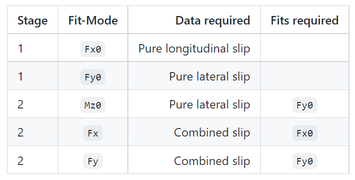
This list is incomplete, as Magic Formula Tire can model more outputs, but this is sufficient for demonstration. This table shows that we should always fit the model to pure slip conditions first (Fx0, Fy0) and then move on to the other equations. The order naturally comes from the dependencies of the equations. Fx uses Fx0 and only applies a scaling term to it, same for Fy. Note that it does not matter whether you fit Fx0 or Fy0 first, same for Fx and Fy. The order described here is also implemented in the fitter, meaning that if you select multiple fit-modes in the GUI, the fitter will proceed in stages.
Building the GUI
My approach to building the GUI was using the custom UI component class provided by MATLAB to develop a modularized application without AppDesigner. Building the app by using custom components makes it very easy to focus only on a part of the app. You can execute individual UI components in isolation and see if any bugs arise. It is not necessary to always run the full app when developing custom UI component classes.
I still use AppDesigner to create Mockups quickly and see if my planned UI looks good, but I prefer not to use it for the final application, as AppDesigner limits my freedom to choose property access levels, preventing me from creating components in loops and more. However, it should be noted that starting with R2021a, you can now use custom UI components in AppDesigner. This might resolve some of the issues I’ve had in the past, but I haven’t tried this yet.
App Demonstration
I will now give a demonstration of the core workflow with data from the FSAE Tire Test Consortium. The data has been obscured and de-identified to conform with the license agreement.
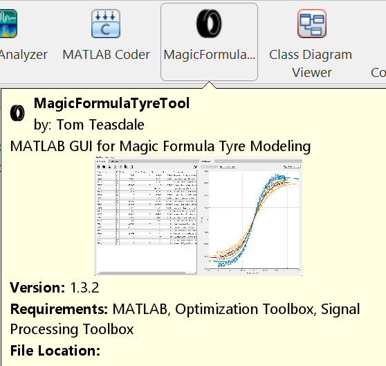
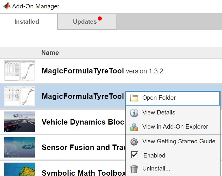
Install the App
There are multiple ways to install the app, but the suggested way is to download it from FileExchange. Alternatively, you can download the latest release from GitHub, but new releases are synced to FileExchange anyway. Download and install the toolbox (*.mltbx) which also includes the app. You can then start the tool from your app catalog.
Import Tire Data
First, we need to acquire measurement data. If you are a member of the FSAE TTC, you can proceed to their forum and download data from there. Please only use data formatted as MAT and in SI units, otherwise, the pre-installed parsers will fail.
In general, TTC data is split into two types of tests
- Drive/Brake
- Cornering
Drive/Brake is a maneuver with either zero slip angle or constant slip angles (steering angles). While all other inputs are held constant, the slip ratio is swept (by driving and braking the tire). Cornering does not consider slip ratio at all and only sweeps slip angle while all other inputs are constant. As you can see, to fit a complete Magic Formula Tire model, you need both the Drive/Brake and Cornering dataset for a given tire. You can follow this example by using the de-identified and obscured data included in the installed toolbox. Simply navigate to the toolbox folder, where you will find example data under doc/examples/fsae-ttc-data/, in case you don’t have access to the TTC (yet). Just keep in mind that the tire characteristics have been modified and the resulting model will behave like a real tire.
Now navigate to the Tyre Data tab and follow the import process as shown.
Configure and Run Fitter
First, we need to create a new tire model. For this, simply navigate back to the Tyre Model tab and click New Model, choose a file to save to and then you should see the following default model.
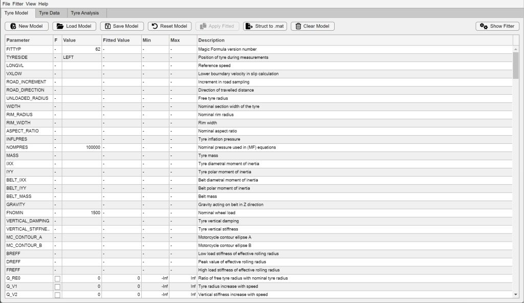
We can navigate to the Tyre Analysis tab and see how well this model fits the data. Spoiler alert: it doesn’t which makes sense, as we haven’t fitted it yet.
Next, we have to configure the fit-modes. A fit-mode in this context is the equation we are going to fit. As explained earlier, different equations require different data to be fitted. For example, fitting Fx0 requires data with no slip angle (pure longitudinal slip). In any case, you should always fit the modes Fx0 and Fy0 first. So let’s do that. Navigating back to the Tyre Model tab, we can adjust the fit-modes and start fitting.
When I noticed that the objective function was decreasing very slowly, I canceled the process. You don’t lose the current state of fmincon though, and the last iteration is saved. Note that I also canceled before Fy0 was fitted, so only Fx0 should have been improved. We can now look at the fitted values and append them to our model.
In case you don’t trust the fitted values, you could also manually transfer them by typing into the value field.
Verify Model-Data-Fit
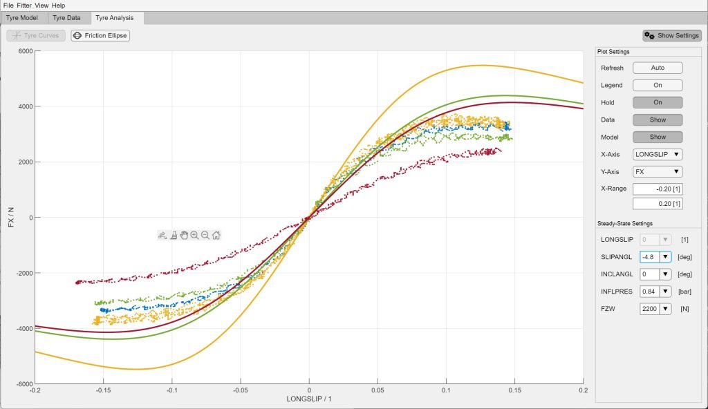
Let us navigate again to the Tyre Analysis tab and plot a few steady-state conditions to verify the model fit.
The fit is not perfect, but satisfactory. Notice that we have not fitted Fy0, Fx and Fy yet, so we should expect bad results for those modes.
Tuning the Model Manually
In case you want to play around with the model and quickly see the results, I suggest changing the window layout and using the Auto-Refresh option of the plot. This is a great way to understand the meaning and effects of the model parameters. It is also a necessary step if your goal is a perfect fit. The fitter is good, but not perfect.
Export Fitted Tire Model
You can now either export the model as a TIR-file which is both great for saving and re-importing the model to the Magic Formula Tire tool, but also the interface to many commercial tools in the market (ADAMS, Siemens NX, Simulink, etc). The exported file will look something like this
…
[LONGITUDINAL_COEFFICIENTS]
PCX1 = 1.6
PDX1 = 1.2
PDX2 = -0.18232
PDX3 = 15
PEX1 = -5.6295e-09
PEX2 = 0.24361
PEX3 = 0
PEX4 = 0
…
Alternatively, you can choose to export as MAT, which will then convert the tire model parameters to a struct and save it to the MAT file. This export makes sense if you need to use the Magic Formula Tire model within MATLAB, using the mftyre.v62.eval function from the library for example.
Note that currently it is not possible to import the MAT file into the tool, so always keep the TIR-file saved apart from the MAT export.
Results and conclusion
We have now fitted our Magic Formula Tire model to real data from the FSAE TTC. The whole process took less than 5 minutes, although we have skipped some steps for demonstration purposes. As mentioned before, you can either use the TIR-file for third-party simulations or use the exported struct in MATLAB directly. If you want to use the Magic Formula Tire MATLAB library, use the following syntax.
[Fx,Fy] = mftyre.v62.eval(p,slipangl,longslip,inclangl,inflpres,FZW,tyreSide)
Where p is the exported parameter struct. In my experience, this evaluation function has proven to be very fast in execution with little overhead. Since it was created for use in real-time control and estimation algorithms in mind, this was a necessary condition.
However, the equations are currently not complete. They don’t calculate the moments Mz0, Mz, Mx and My for example. Also, the turn slip has been neglected. As a great alternative, you can also use the popular mfeval project created by Marco Furlan to evaluate the exported TIR-file. Just keep in mind that the GUI also doesn’t fit the modes mentioned.
output = mfeval(TIRfile, inputs, useMode);
I hope that this tool can benefit some students in Formula Student to finally create a detailed tire model themselves!
Future scope
The Magic Formula Tire Tool seems to be working great already I have been told by a few beta-testers. But there are still some features planned for the near future.
- Compatibility with older versions of Magic Formula Tire
- More Analysis options (e.g. Kamm-Circle)
- Quality-of-Life improvements (usability)
- Weighting functions for Fitter (putting more weight on lower loads for example)
If you want to be kept in the loop, consider starring my GitHub repository or rating my tool on FileExchange. Both will keep me motivated to add features to the tool. In case you want to contribute yourself, please feel free to do so. Get in touch with me and we will find a way to collaborate!
Acknowledgments
This project would not have been possible without the data provided by the Formula SAE Tire Test Consortium (FSAE TTC) and the Calspan Tire Testing Research Facility (TIRF). De-identified and obscured test data has been used in examples and images or recordings of the application, to conform to the license agreement. Special thanks to Dr. Edward M. Kasprzak for granting me permission to provide the user, de-identified and obscured data for demonstration purposes.
I also want to acknowledge Marco Furlan with whom I had an enjoyable exchange on LinkedIn. He developed the mentioned mfeval toolbox, which is still the definitive open-source MATLAB implementation of Magic Formula Tire on the market. His project helped me get started with Magic Formula Tire almost three years back and was greatly appreciated.
Lastly, I want to acknowledge the previously reference blog post by MathWorks staff called Analyzing Tire Test Data from which I learned the genius way of using the MATLAB function histcounts to automatically separate time series data into steady-states. Their technique has been used to develop the measurement import parsers.
- Category:
- Automotive


Comments
To leave a comment, please click here to sign in to your MathWorks Account or create a new one.