
MathWorks Logo, Part Two. Finite Differences
After reviewing the state of affairs fifty years ago, I use classic finite difference methods, followed by extrapolation, to find the first eigenvalue of the region underlying the MathWorks logo.
Contents
Fifty Years Ago
My Ph. D. dissertation, submitted to the Stanford Math Department in 1965, was titled "Finite Difference Methods for Eigenvalues of Laplace's Operator". The thesis was not just about the L-shaped region, but the L was my primary example.
My thesis advisor was George Forsythe, who had investigated the L in some of his own research. At the time, many people were interested in methods for obtaining guaranteed upper and lower bounds for eigenvalues of differential operators. Forsythe had shown that certain kinds of finite difference methods could provide lower bounds for convex regions. But the L is not convex, so that made it a region to investigate.
Nobody knew the first eigenvalue very precisely. Forsythe and Wolfgang Wasow published a book in 1960, "Finite Difference Methods for Partial Differential Equations" (John Wiley & Sons), that features the L in several different sections. In section 24.3 Forsythe references some calculations he had done in 1954 that led him to estimate that
$$ \lambda_1 = 9.636 $$
He goes on to report an informal conjecture made in the late '50s from his colleague R. De Vogelaere that
$$ 9.63968 < \lambda_1 < 9.63972 $$
I repeat these numbers here to give you some idea of the accuracy we were working with back then. We will see in a later post that the right answer is just outside De Vogelaere's upper bound.
My Calculations in 1964

Here's a page from my thesis. The contour plot at the bottom of the page would eventually evolve into the MathWorks logo. The plot was made on a Calcomp plotter, which involved a computer controlled solenoid holding a ball-point or liquid ink pen moving across a paper rolled on a rotating drum. This was a very effective device and was used in computer centers worldwide for a number of years.
The calculations shown on this page are the first eigenvalue of the finite difference Laplacian for ten values of the mesh size $h$. The finest mesh, $h$ = 1/100, has 29,601 interior points. As I recall, the calculation of the first eigenvalue, which I did with a kind of inverse power method, took about half an hour on Stanford's campus main frame, an IBM 7090.
Here is a plot of these values I computed fifty years ago. I've added a black line at what we now know to be the limiting value, the first eigenvalue of the continuous differential operator. You can see that the finite difference values are converging quite slowly. Furthermore, they are converging from above. Forsythe was not going to get his lower bound for this nonconvex region.
thesis_graph
Slow Convergence
The show rate of convergence of the finite difference eigenvalue with decreasing mesh size is caused by the fact that the corresponding eigenfunction is singular at the reentrant corner in the region. The gradient becomes infinite at that corner. You can see the contour lines crowding together near the corner. If you tried to make a drum head or tambourine by stretching a membrane over an L-shaped frame, it would rip.
To be more precise, use polar coordinates, $r$ and $\theta$, centered at the reentrant corner. Note that to cover the interior of the region $\theta$ will run from $0$ to $\frac{3}{2}\pi$. It turns out that approaching the corner the first eigenfunction has the asymptotic behavior
$$ u(r,\theta) \approx r^\alpha \sin{\alpha \theta} $$
with $\alpha = \frac{2}{3}$. This implies that the $k$ -th derivatives of the eigenfunction have singularities that behave like
$$ \partial^k u \approx r^{\alpha-k} $$
When this fact is combined with the Taylor series analysis of the discretization error of the five-point finite difference operator we find that the first eigenvalue converges at the rate
$$ \lambda_{1,h} - \lambda_1 \approx O(h^{2 \alpha}) = O(h^\frac{4}{3}) $$
This is significantly slower than the $O(h^2)$ convergence rate obtained when the eigenfunction is not singular.
Difference Methods in MATLAB
Now let's use my laptop and the sparse capabilities in MATLAB. The functions numgrid, delsq, spy, and eigs have been included in the sparfun directory since its introduction. We begin by generating a small L-shaped numbering scheme.
   n = 10;
   L = numgrid('L',n+1)
L =
     0     0     0     0     0     0     0     0     0     0     0
     0     1     5     9    13    17    21    30    39    48     0
     0     2     6    10    14    18    22    31    40    49     0
     0     3     7    11    15    19    23    32    41    50     0
     0     4     8    12    16    20    24    33    42    51     0
     0     0     0     0     0     0    25    34    43    52     0
     0     0     0     0     0     0    26    35    44    53     0
     0     0     0     0     0     0    27    36    45    54     0
     0     0     0     0     0     0    28    37    46    55     0
     0     0     0     0     0     0    29    38    47    56     0
     0     0     0     0     0     0     0     0     0     0     0
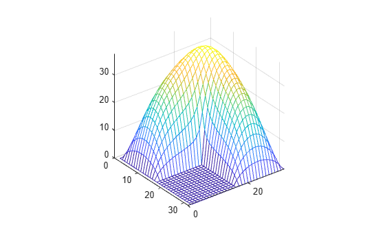
To illustrate how this scheme works, superimpose it on a finite difference grid.
Lgrid(L)
The statement
A = delsq(L);
constructs matrix representation of the five-point discrete Laplacian for the grid L.
   whos A
   issym = isequal(A,A')
   nnzA = nnz(A)
  Name       Size            Bytes  Class     Attributes

  A         56x56             3156  double    sparse

issym =
     1
nnzA =
   244
So for this grid, the discrete Laplacian A is a 56-by-56 sparse double precision symmetric matrix with 244 nonzero elements. That's an average of
ratio = nnz(A)/size(A,1)
ratio =
    4.3571
nonzero elements per row. Each interior grid point is connected to its four nearest neighbors. For example, point number 44 is connected to points 35, 43, 45, and 53. So the nonzero elements in column 44 are
A(:,44)
ans =
  (35,1)       -1
  (43,1)       -1
  (44,1)        4
  (45,1)       -1
  (53,1)       -1
There are 4's on the diagonal and -1's is positions on the off-diagonals corresponding to connections between neighbors. They can be seen in the spy plot which shows the location of the nonzeros.
spy(A)
Scale A by the square of the mesh size and then use eigs to find its five smallest eigenvalues.
   h = 2/n
   A = A/h^2;
   eigvals = eigs(A,5,'sm')
h =
    0.2000
eigvals =
   30.3140
   27.7177
   19.0983
   14.6708
    9.6786
My Calculations in 2014
Run for decreasing mesh size, up to the memory capacity of my laptop.
type L_finite_diffs
% L_finite_diffs
% Script for MathWorks Logo, Part Two
% Finite Differences

   opts.tol = 1.0e-12;
   eigvals = zeros(13,5);
   tic
   for n = 50:50:650
      L = numgrid('L',n+1);
      h = 2/n;
      A = delsq(L)/h^2;
      e = eigs(A,5,'sm',opts);
      eigvals(n/50,:) = fliplr(e');
      fprintf('%4.0f %10.6f %9.0f %10.0f %16.12f\n', ...
         n,h,size(A,1),nnz(A),e(5))
   end
   toc
   save eigvals eigvals
type L_finite_diffs_results
     n       h       size(A)    nnz(A)     lambda_1,h

     50  0.040000      1776       8684   9.661331286788
    100  0.020000      7301      36109   9.649547111146
    150  0.013333     16576      82284   9.645736333124
    200  0.010000     29601     147209   9.643932372382
    250  0.008000     46376     230884   9.642903412412
    300  0.006667     66901     333309   9.642247498956
    350  0.005714     91176     454484   9.641797238078
    400  0.005000    119201     594409   9.641471331746
    450  0.004444    150976     753084   9.641225852818
    500  0.004000    186501     930509   9.641035124947
    550  0.003636    225776    1126684   9.640883203502
    600  0.003333    268801    1341609   9.640759699387
    650  0.003077    315576    1575284   9.640657572983

   Elapsed time is 29.729023 seconds.
Extrapolation
I know the Taylor series analysis of the discretization error involves terms with both $h^{4/3}$ and $h^2$, so let's use these as the basis for extrapolation. Use backslash to do a least squares fit.
   load eigvals
   eigvals = eigvals(:,1);
   n = (50:50:650)';
   h = 2./n;
   e = ones(size(h));
   X = [e h.^(4/3) h.^2];
   c = X(4:end,:)\eigvals(4:end);
   lambda1 = c(1);

   n = (50:10:650)';
   h = 2./n;
   fit = c(1) + c(2)*h.^(4/3) + c(3)*h.^2;
   plot(n(1:5:end),eigvals,'o',n,fit,'-',[0 700],[lambda1 lambda1],'k-')
   set(gca,'xtick',100:100:600,'xticklabel',...
      num2str(sprintf('2/%3.0f\n',100:100:600)))
   xlabel('h')
Frankly, I was surprised when the extrapolation of the finite difference eigenvalues produced this result.
   format long
   lambda1
lambda1 =
   9.639723753239963
I know from techniques that I will describe in later posts that this agrees with the exact eigenvalue of the continuous differential operator to seven decimal places. Before I wrote this blog I never tried this computation on computers with enough memory to handle meshes this fine and was never able to obtain this kind of accuracy from extrapolated finite difference eigenvalues.
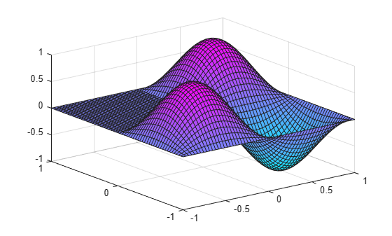
Eigenfunction
Let's do a contour plot of the eigenfunction. The tricky part is using the grid numbering in L to insert the eigenvector back onto the grid.
   close
   n = 100;
   h = 2/n;
   L = numgrid('L',n+1);
   A = delsq(L)/h^2;
   [V,E] = eigs(A,5,'sm');
   L(L>0) = -V(:,5);
   contourf(fliplr(L),12);
   axis square
   axis off
The plot shows off parula, the MATLAB default colormap with Handle Graphics II and Release 2014b. The colormap derives its name from the parula, which is a small warbler found throughout eastern North America that exhibits these colors. As our contour plot demonstrates, the color intensity varies smooth and uniformly as the contour levels increase. This is not true of jet, the old default. Steve Eddins has more about parula in his blog.


댓글
댓글을 남기려면 링크 를 클릭하여 MathWorks 계정에 로그인하거나 계정을 새로 만드십시오.