This post is by my colleague Cosmin Ionita.

The 'makima' cubic interpolation method was recently introduced in MATLAB® in the R2017b release as a new option in interp1, interp2, interp3, interpn, and griddedInterpolant. Its implementation is not user visible; thus, we have been receiving inquiries from our users about the specifics of this new cubic method.

In the following, we address our users' inquiries by answering these questions:

In a nutshell, 'makima' is short for modified Akima piecewise cubic Hermite interpolation. It represents a MATLAB-specific modification of Akima's derivative formula and has the following key properties:

Contents

Akima piecewise cubic Hermite interpolation

For each interval $[x_i~x_{i+1})$ of an input data set of nodes $x$ and values $v$, piecewise cubic Hermite interpolation finds a cubic polynomial which not only interpolates the given data values $v_i$ and $v_{i+1}$ at the interval's nodes $x_i$ and $x_{i+1}$, but also has specific derivatives $d_i$ and $d_{i+1}$ at $x_i$ and $x_{i+1}$. For more details we refer to the interpolation chapter in Cleve's Numerical Computing with MATLAB textbook.

The key to cubic Hermite interpolation is the choice of derivatives $d_i$.

In his 1970 paper, Hiroshi Akima introduced a derivative formula which avoids excessive local undulations:

H. Akima, "A New Method of Interpolation and Smooth Curve Fitting Based on Local Procedures", JACM, v. 17-4, p.589-602, 1970.

Let $\delta_i =\left(v_{i+1} -v_i \right)/\left(x_{i+1} -x_i \right)$ be the slope of the interval $[x_i~x_{i+1})$. Akima's derivative at $x_i$ is defined as:

$$d_i = \frac{|\delta_{i+1} - \delta_i|\delta_{i-1} + |\delta_{i-1} - \delta_{i-2}|\delta_i} {|\delta_{i+1} - \delta_i| + |\delta_{i-1} - \delta_{i-2}|},$$

and represents a weighted average between the slopes $\delta_{i-1}$ and $\delta_i$ of the intervals $[x_{i-1}~x_i)$ and $[x_i~x_{i+1})$:

$$d_i = \frac{w_1}{w_1+w_2}\delta_{i-1} + \frac{w_2}{w_1+w_2}\delta_i \,, \quad\quad w_1 = |\delta_{i+1} - \delta_i|, \quad\quad w_2 = |\delta_{i-1} - \delta_{i-2}|.$$

Notice that Akima's derivative at $x_i$ is computed locally from the five points $x_{i-2}$, $x_{i-1}$, $x_i$, $x_{i+1}$, and $x_{i+2}$. For the end points $x_1$ and $x_n$, it requires the slopes $\delta_{-1}, \delta_0$ and $\delta_n ,\delta_{n+1}$. Since these slopes are not available in the input data, Akima proposed using quadratic extrapolation to compute them as $\delta_0 = 2\delta_1 -\delta_2$, $\delta_{-1} = 2\delta_0 -\delta_1$ and $\delta_n = 2\delta_{n-1} -\delta_{n-2}$, $\delta_{n+1} = 2\delta_n -\delta_{n-1}$.

But wait!

MATLAB already has two cubic Hermite interpolation methods (see Cleve's blog Splines and Pchips):

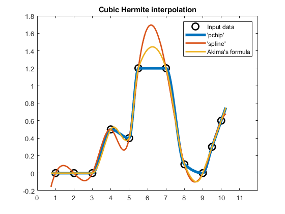
How does Akima's formula compare with 'spline' and 'pchip'?

Akima's formula finds a nice middle ground between 'spline' and 'pchip':

Here's a representative example comparing these three cubic Hermite interpolants:

    x1 = [1 2 3 4 5 5.5 7 8 9 9.5 10];
    v1 = [0 0 0 0.5 0.4 1.2 1.2 0.1 0 0.3 0.6];
    xq1 = 0.75:0.05:10.25;
    compareCubicPlots(x1,v1,xq1,false,'NE')

Modified Akima interpolation -- 'makima'

Akima's formula certainly produces nice results. However, we are not yet ready to fully adopt it.

Edge case of equal side slopes

When the lower slopes are equal, $\delta_{i-2} =\delta_{i-1}$, and the upper slopes are equal, $\delta_i =\delta_{i+1}$, both the numerator and denominator become equal to 0 and Akima's formula returns NaN. Akima himself recognized this problem and proposed taking the average of the lower and upper slopes for this edge case: $d_i =\left(\delta_{i-1} +\delta_i \right)/2$.

Let's try this fix for the following data set where the intervals $[3~4)$ and $[4~5)$ have equal slopes $\delta_3 =\delta_4 =1$ and the intervals $[5~6)$ and $[6~7)$ also have equal slopes $\delta_5 =\delta_6 =0$:

    x2 = 1:8;
    v2 = [-1 -1 -1 0 1 1 1 1];
    xq2 = 0.75:0.05:8.25;
    compareCubicPlots(x2,v2,xq2,false,'SE')
    ylim([-1.2 1.2])

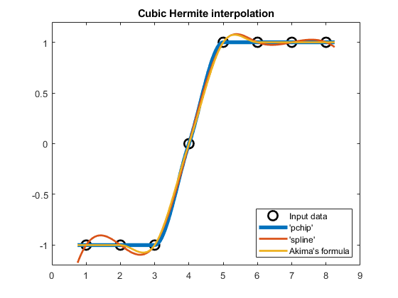
In this case, Akima's NaN derivative at $x_5=5$ gets replaced with the average slope $d_5 =\left(\delta_4 +\delta_5 \right)/2=0.5$.

But we are still not ready!

When should we switch from Akima's formula to the averaging formula? What if the slopes are almost equal?

Let's change the above example such that $\delta_5 =\varepsilon$ and $\delta_6 =-\varepsilon$ by setting $v_6 =1+\varepsilon$ , where $\varepsilon =2^{-52}$ represents machine epsilon. We can now compare Akima's full formula with the averaging formula at $d_5$ for two data sets that differ only by $\varepsilon$:

% v2eps: new data set which differs only by an eps in v2(6)
    v2eps = v2; v2eps(6) = v2eps(6) + eps;

    plot(x2,v2,'ko','LineWidth',2,'MarkerSize',10,'DisplayName','Input data v2')
    hold on
    plot(xq2,akima(x2,v2,xq2),'Color',[1 2/3 0],'LineWidth',2,...
        'DisplayName','v2(6) = 1 uses averaging formula')
    plot(xq2,akima(x2,v2eps,xq2),'-.','Color',[1 2/3 0],'LineWidth',2,...
        'DisplayName','v2(6) = 1+eps uses Akima''s formula')
    hold off
    legend('Location','SE')
    title('Akima interpolant for (almost) equal side slopes' )
    ylim([-1.2 1.2])

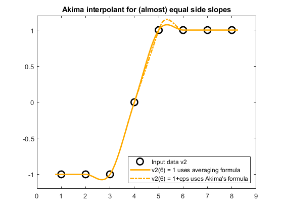
The averaging formula (solid line) returns the derivative $d_5=0.5$ while Akima's formula (dashed line) returns $d_5=1$. Therefore, there is an unwanted non-negligible difference at around $x_5=5$ between the two Akima interpolants, even though the two underlying data sets differ only by $\varepsilon$ at $v_6$.

Requirement (1)

We do not want our Akima interpolant to switch to a different formula for edge cases.

Overshoot if data is constant for more than two consecutive nodes

The previous example was strategically chosen to also reveal another property of the Akima interpolant: if the data is constant for more than two consecutive nodes, like $v_5=v_6=v_7=1$ in the previous example, then the Akima interpolant may produce an overshoot, namely, the interpolant's undulation in the $[5~6)$ interval above.

This special type of overshoot is not desirable in many engineering applications.

The same concerns hold for the undershoot present in the $[2~3)$ interval above.

Requirement (2)

We do not want our Akima interpolant to produce overshoot (or undershoot) when the data is constant for more than two consecutive nodes.

Modified Akima formula

In MATLAB, 'makima' cubic Hermite interpolation addresses requirements (1) and (2) outlined above.

To eliminate overshoot and avoid edge cases of both numerator and denominator being equal to 0, we modify Akima's derivative formula by tweaking the weights $w_1$ and $w_2$ of the slopes $\delta_{i-1}$ and $\delta_i$:

$$ d_i = \frac{w_1}{w_1+w_2}\delta_{i-1} + \frac{w_2}{w_1+w_2}\delta_i \,, \quad\quad w_1 = |\delta_{i+1} - \delta_i| + |\delta_{i+1} + \delta_i|/2, \quad\quad w_2 = |\delta_{i-1} - \delta_{i-2}| + |\delta_{i-1} + \delta_{i-2}| / 2. $$

This modified formula represents the 'makima' derivative formula used in MATLAB:

Let's try the 'makima' formula on the above overshoot example:

    compareCubicPlots(x2,v2,xq2,true,'SE')
    ylim([-1.2 1.2])

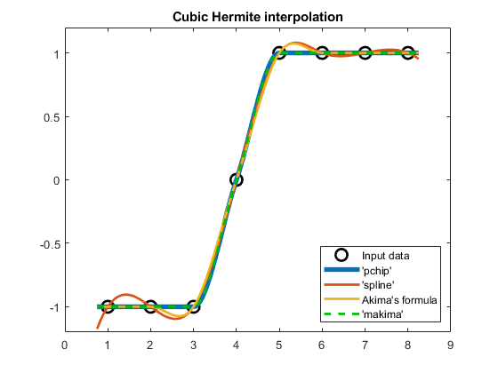
Indeed, 'makima' does not produce an overshoot if the data is constant for more than two nodes ($v_5=v_6=v_7=1$ above).

But what does this mean for the undulations we saw in our first example?

    compareCubicPlots(x1,v1,xq1,true,'NE')

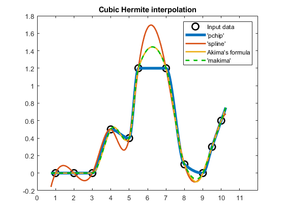
Notice that 'makima' closely follows the result obtained with Akima's formula. In fact, the results are so similar that it is hard to tell them apart on the plot.

Therefore, 'makima' still preserves Akima's desirable properties of being a nice middle ground between 'spline' and 'pchip' in terms of the resulting undulations.

Generalization to n-D grids

But we are still not done!

Akima's formula and our modified 'makima' formula have another desirable property: they generalize to higher dimensional n-D gridded data. Akima noticed this property in his 1974 paper.

H. Akima, "A Method of Bivariate Interpolation and Smooth Surface Fitting Based on Local Procedures", Communications of the ACM, v. 17-1, p.18-20, 1974.

For example, to interpolate on a 2-D grid $\left(x,y\right)$, we first apply the 'makima' derivative formula separately along $x$ and $y$ to obtain two directional derivatives for each grid node. Then, we also compute the cross-derivative along $xy$ for each grid node. The cross-derivative formula first computes the 2-D divided differences corresponding to the 2-D grid data and applies the 'makima' derivative formula along $x$ on these differences; then, it takes the result and applies the derivative formula along $y$. The derivatives and cross-derivatives are then plugged in as coefficients of a two-variable cubic Hermite polynomial representing the 2-D interpolant.

The same procedure applies to higher dimensional n-D grids with $n\ge 2$ and requires computing cross-derivatives along all possible cross-directions. Therefore, 'makima' is supported not only in interp1, but also in interp2, interp3, interpn, and griddedInterpolant.

Here's how 2-D 'makima' interpolation compares with 2-D 'spline' interpolation on gridded data generated with the peaks function:

    [X1,Y1,V1] = peaks(5);
    [Xq1,Yq1] = meshgrid(-3:0.1:3,-3:0.1:3);

    Vqs1 = interp2(X1,Y1,V1,Xq1,Yq1,'spline');
    surf(Xq1,Yq1,Vqs1)
    axis tight
    title('2-D ''spline''')
    snapnow

    Vqm1 = interp2(X1,Y1,V1,Xq1,Yq1,'makima');
    surf(Xq1,Yq1,Vqm1)
    axis tight
    title('2-D ''makima''')

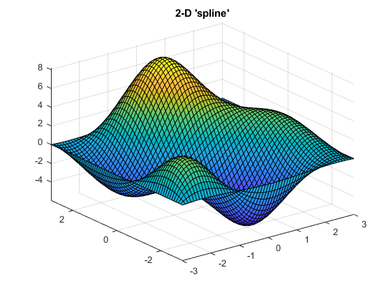
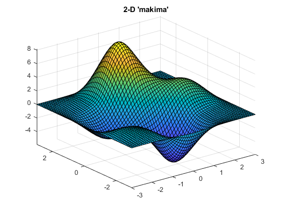
Notice the smaller undulations (or wiggles) generated by 'makima'.

Finally, let's try 'makima' on an example with a few 2-D peaks where the data has sharp edges and steps:

    V2 = zeros(10);
    V2(2:5,2:5) = 3/7; % First step
    V2(6:7,6:7) = [1/4 1/5; 1/5 1/4]; % Middle step
    V2(8:9,8:9) = 1/2; % Last step
    V2 = flip(V2,2);
    [Xq2,Yq2] = meshgrid(1:0.2:10,1:0.2:10);

    Vqs2 = interp2(V2,Xq2,Yq2,'spline');
    surf(Xq2,Yq2,Vqs2)
    axis tight
    title('2-D ''spline''')
    snapnow

    Vqm2 = interp2(V2,Xq2,Yq2,'makima');
    surf(Xq2,Yq2,Vqm2)
    axis tight
    title('2-D ''makima''')

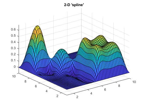
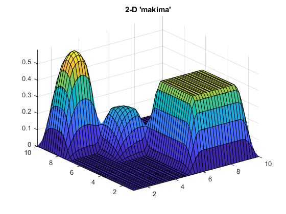
The 'makima' result has smaller undulations (or wiggles) than 'spline'.

Summary

We conclude with a summary of properties of interest for the three cubic Hermite interpolation methods supported in MATLAB:

    summary = table( ...
        ["C2"; "Uses all points"; "Not-a-knot condition"; "Yes"], ...
        ["C1"; "Uses 4 points"; "One-sided slope"; "No"], ...
        ["C1"; "Uses 5 points"; "Quadratic extrapolation"; "Yes"], ...
        'VariableNames', ...
        ["spline" "pchip" "makima"], ...
        'RowNames', ...
        ["Continuity"; "Locality"; "End points"; "Supports n-D"]);
    disp(summary)

                            spline                  pchip                   makima          
                    ______________________    _________________    _________________________
    Continuity      "C2"                      "C1"                 "C1"                     
    Locality        "Uses all points"         "Uses 4 points"      "Uses 5 points"          
    End points      "Not-a-knot condition"    "One-sided slope"    "Quadratic extrapolation"
    Supports n-D    "Yes"                     "No"                 "Yes"                    

code

compareCubicPlots

function compareCubicPlots(x,v,xq,showMakima,legendLocation)
% Plot 'pchip', 'spline', Akima, and 'makima' interpolation results
    vqp = pchip(x,v,xq);      % same as vq = interp1(x,v,xq,'pchip')
    vqs = spline(x,v,xq);     % same as vq = interp1(x,v,xq,'spline')
    vqa = akima(x,v,xq);
    if showMakima
        vqm = makima(x,v,xq); % same as vq = interp1(x,v,xq,'makima')
    end

    plot(x,v,'ko','LineWidth',2,'MarkerSize',10,'DisplayName','Input data')
    hold on
    plot(xq,vqp,'LineWidth',4,'DisplayName','''pchip''')
    plot(xq,vqs,'LineWidth',2,'DisplayName','''spline''')
    plot(xq,vqa,'LineWidth',2,'DisplayName','Akima''s formula')
    if showMakima
        plot(xq,vqm,'--','Color',[0 3/4 0],'LineWidth',2, ...
            'DisplayName','''makima''')
    end
    hold off
    xticks(x(1)-1:x(end)+1)
    legend('Location',legendLocation)
    title('Cubic Hermite interpolation')
end

akima

function vq = akima(x,v,xq)
%AKIMA   Akima piecewise cubic Hermite interpolation.
%
%   vq = AKIMA(x,v,xq) interpolates the data (x,v) at the query points xq
%   using Akima's cubic Hermite interpolation formula.
%
%   References:
%
%       H. Akima, "A New Method of Interpolation and Smooth Curve Fitting
%       Based on Local Procedures", JACM, v. 17-4, p.589-602, 1970.
%
%   AKIMA vs. PCHIP vs. SPLINE:
%
%     - Akima's cubic formula is a middle ground between SPLINE and PCHIP:
%       It has lower-amplitude wiggles than SPLINE, but is not as agressive
%       at reducing the wiggles as PCHIP.
%     - Akima's cubic formula and SPLINE generalize to n-D grids.
%
%   Example: Compare AKIMA with MAKIMA, SPLINE, and PCHIP
%
%       x = [1 2 3 4 5 5.5 7 8 9 9.5 10];
%       v = [0 0 0 0.5 0.4 1.2 1.2 0.1 0 0.3 0.6];
%       xq = 0.75:0.05:10.25;
%       vqs = spline(x,v,xq);
%       vqp = pchip(x,v,xq);
%       vqa = akima(x,v,xq);
%       vqm = makima(x,v,xq);
%
%       figure
%       plot(x,v,'ko','LineWidth',2,'MarkerSize',10), hold on
%       plot(xq,vqp,'LineWidth',4)
%       plot(xq,vqs,xq,vqa,xq,vqm,'--','LineWidth',2)
%       legend('Data','''pchip''','''spline''','Akima''s formula','''makima''')
%       title('Cubic Hermite interpolation in MATLAB')
%
%   See also MAKIMA, SPLINE, PCHIP.


%   mailto: cosmin.ionita@mathworks.com

    assert(isvector(x) && isvector(v) && (numel(x) == numel(v)))
    assert(numel(x) > 2)
    x = x(:).'; v = v(:).'; % Same shapes as in pchip.m and spline.m

    % Compute Akima slopes
    h = diff(x);
    delta = diff(v)./h;
    slopes = akimaSlopes(delta);

    % Evaluate the piecewise cubic Hermite interpolant
    vq = ppval(pwch(x,v,slopes,h,delta),xq);
end

akimaSlopes

function s = akimaSlopes(delta)
% Derivative values for Akima cubic Hermite interpolation

% Akima's derivative estimate at grid node x(i) requires the four finite
% differences corresponding to the five grid nodes x(i-2:i+2).
%
% For boundary grid nodes x(1:2) and x(n-1:n), append finite differences
% which would correspond to x(-1:0) and x(n+1:n+2) by using the following
% uncentered difference formula correspondin to quadratic extrapolation
% using the quadratic polynomial defined by data at x(1:3)
% (section 2.3 in Akima's paper):
    n = numel(delta) + 1; % number of grid nodes x
    delta_0  = 2*delta(1)   - delta(2);
    delta_m1 = 2*delta_0    - delta(1);
    delta_n  = 2*delta(n-1) - delta(n-2);
    delta_n1 = 2*delta_n    - delta(n-1);
    delta = [delta_m1 delta_0 delta delta_n delta_n1];

% Akima's derivative estimate formula (equation (1) in the paper):
%
%       H. Akima, "A New Method of Interpolation and Smooth Curve Fitting
%       Based on Local Procedures", JACM, v. 17-4, p.589-602, 1970.
%
% s(i) = (|d(i+1)-d(i)| * d(i-1) + |d(i-1)-d(i-2)| * d(i))
%      / (|d(i+1)-d(i)|          + |d(i-1)-d(i-2)|)
    weights = abs(diff(delta));
    weights1 = weights(1:n);   % |d(i-1)-d(i-2)|
    weights2 = weights(3:end); % |d(i+1)-d(i)|
    delta1 = delta(2:n+1);     % d(i-1)
    delta2 = delta(3:n+2);     % d(i)

    weights12 = weights1 + weights2;
    s = (weights2./weights12) .* delta1 + (weights1./weights12) .* delta2;

% To avoid 0/0, Akima proposed to average the divided differences d(i-1)
% and d(i) for the edge case of d(i-2) = d(i-1) and d(i) = d(i+1):
    ind = weights1 == 0 & weights2 == 0;
    s(ind) = (delta1(ind) + delta2(ind)) / 2;
end

makima

function vq = makima(x,v,xq)
%MAKIMA   Modified Akima piecewise cubic Hermite interpolation.
%
%       We modify Akima's formula to eliminate overshoot and undershoot
%       when the data is constant for more than two consecutive nodes.
%
%   vq = MAKIMA(x,v,xq) interpolates the data (x,v) at the query points xq
%   using a modified Akima cubic Hermite interpolation formula.
%
%   References:
%
%       H. Akima, "A New Method of Interpolation and Smooth Curve Fitting
%       Based on Local Procedures", JACM, v. 17-4, p.589-602, 1970.
%
%   MAKIMA vs. PCHIP vs. SPLINE:
%
%     - MAKIMA is a middle ground between SPLINE and PCHIP:
%       It has lower-amplitude wiggles than SPLINE, but is not as agressive
%       at reducing the wiggles as PCHIP.
%     - MAKIMA and SPLINE generalize to n-D grids.
%
%   Example: No overshoot and undershoot with MAKIMA when the data is
%            constant for more than two consecutive nodes
%
%       x = 1:7;
%       v = [-1 -1 -1 0 1 1 1];
%       xq = 0.75:0.05:7.25;
%       vqs = spline(x,v,xq);
%       vqp = pchip(x,v,xq);
%       vqa = akima(x,v,xq);
%       vqm = makima(x,v,xq);
%
%       figure
%       plot(x,v,'ko','LineWidth',2,'MarkerSize',10), hold on
%       plot(xq,vqp,'LineWidth',4)
%       plot(xq,vqs,xq,vqa,xq,vqm,'LineWidth',2)
%       legend('Data','''pchip''','''spline''','Akima''s formula',...
%           '''makima''','Location','SE')
%       title('''makima'' has no overshoot in x(1:3) and x(5:7)')
%
%   Example: Compare MAKIMA with AKIMA, SPLINE, and PCHIP
%
%       x = [1 2 3 4 5 5.5 7 8 9 9.5 10];
%       v = [0 0 0 0.5 0.4 1.2 1.2 0.1 0 0.3 0.6];
%       xq = 0.75:0.05:10.25;
%       vqs = spline(x,v,xq);
%       vqp = pchip(x,v,xq);
%       vqa = akima(x,v,xq);
%       vqm = makima(x,v,xq);
%
%       figure
%       plot(x,v,'ko','LineWidth',2,'MarkerSize',10), hold on
%       plot(xq,vqp,'LineWidth',4)
%       plot(xq,vqs,xq,vqa,xq,vqm,'--','LineWidth',2)
%       legend('Data','''pchip''','''spline''','Akima''s formula','''makima''')
%       title('Cubic Hermite interpolation in MATLAB')
%
%   See also AKIMA, SPLINE, PCHIP.


%   mailto: cosmin.ionita@mathworks.com

    assert(isvector(x) && isvector(v) && (numel(x) == numel(v)))
    assert(numel(x) > 2)
    x = x(:).'; v = v(:).'; % Same shapes as in pchip.m and spline.m

% Compute modified Akima slopes
    h = diff(x);
    delta = diff(v)./h;
    slopes = makimaSlopes(delta);

% Evaluate the piecewise cubic Hermite interpolant
    vq = ppval(pwch(x,v,slopes,h,delta),xq);

end

makimaSlopes

function s = makimaSlopes(delta)
% Derivative values for modified Akima cubic Hermite interpolation

% Akima's derivative estimate at grid node x(i) requires the four finite
% differences corresponding to the five grid nodes x(i-2:i+2).
%
% For boundary grid nodes x(1:2) and x(n-1:n), append finite differences
% which would correspond to x(-1:0) and x(n+1:n+2) by using the following
% uncentered difference formula correspondin to quadratic extrapolation
% using the quadratic polynomial defined by data at x(1:3)
% (section 2.3 in Akima's paper):
    n = numel(delta) + 1; % number of grid nodes x
    delta_0  = 2*delta(1)   - delta(2);
    delta_m1 = 2*delta_0    - delta(1);
    delta_n  = 2*delta(n-1) - delta(n-2);
    delta_n1 = 2*delta_n    - delta(n-1);
    delta = [delta_m1 delta_0 delta delta_n delta_n1];

% Akima's derivative estimate formula (equation (1) in the paper):
%
%       H. Akima, "A New Method of Interpolation and Smooth Curve Fitting
%       Based on Local Procedures", JACM, v. 17-4, p.589-602, 1970.
%
% s(i) = (|d(i+1)-d(i)| * d(i-1) + |d(i-1)-d(i-2)| * d(i))
%      / (|d(i+1)-d(i)|          + |d(i-1)-d(i-2)|)
%
% To eliminate overshoot and undershoot when the data is constant for more
% than two consecutive nodes, in MATLAB's 'makima' we modify Akima's
% formula by adding an additional averaging term in the weights.
% s(i) = ( (|d(i+1)-d(i)|   + |d(i+1)+d(i)|/2  ) * d(i-1) +
%          (|d(i-1)-d(i-2)| + |d(i-1)+d(i-2)|/2) * d(i)  )
%      / ( (|d(i+1)-d(i)|   + |d(i+1)+d(i)|/2  ) +
%          (|d(i-1)-d(i-2)| + |d(i-1)+d(i-2)|/2)
    weights = abs(diff(delta)) + abs((delta(1:end-1)+delta(2:end))/2);

    weights1 = weights(1:n);   % |d(i-1)-d(i-2)|
    weights2 = weights(3:end); % |d(i+1)-d(i)|
    delta1 = delta(2:n+1);     % d(i-1)
    delta2 = delta(3:n+2);     % d(i)

    weights12 = weights1 + weights2;
    s = (weights2./weights12) .* delta1 + (weights1./weights12) .* delta2;

% If the data is constant for more than four consecutive nodes, then the
% denominator is zero and the formula produces an unwanted NaN result.
% Replace this NaN with 0.
    s(weights12 == 0) = 0;
end

Copyright 2019 The MathWorks, Inc.
Get the MATLAB code

Published with MATLAB® R2018b