Introduction to the New MATLAB Data Types in R2013b
Today I’d like to introduce a fairly frequent guest blogger Sarah Wait Zaranek who works for the MATLAB Marketing team here at The MathWorks. She and I will be writing about the new capabilities for MATLAB in R2013b. In particular, there are two new data types in MATLAB in R2013b – table and categorical arrays.
Contents
- What are Tables and Categorical Arrays?
- Importing Data into a Table
- Looking at Variable Names (Column Names)
- Accessing the Data in Your Table
- Converting Data to Categorical Arrays
- Creating a New Table
- Adding/Removing Variables
- Removing Missing Data
- Summarizing a Table
- Sorting Data
- Applying Functions to Table Variables
- Joining (Merging) Tables
- Plotting Data From the Final Table
- Your Thoughts?
What are Tables and Categorical Arrays?
Table is a new data type suitable for holding heterogenous data and metadata. Specifically, tables are useful for mixed-type tabular data that are often stored as columns in a text file or in a spreadsheet. Tables consist of rows and column-oriented variables. Categorical arrays are useful for holding categorical data - which have values from a finite list of discrete categories.
One of the best ways to learn more about tables and categorical arrays is to see them in action. So, in this post, we will use tables and categoricals to examine some airplane flight delay data. The flight data is freely available from the Bureau of Transportation Statistics (BTS). You can download it yourself here. The weather data is from the National Climatic Data Center (NCDC) and is available here.
Importing Data into a Table
You can import your data into a table interactively using the Import Tool or you can do it programmatically, using readtable.
FlightData = readtable('Jan2010Flights.csv');

whos FlightData
  Name                Size              Bytes  Class    Attributes

  FlightData      17816x7             9007742  table
The entire contents of the file are now contained in a single variable – a table. Here you are reading in your data from a csv file. readtable also supports reading from .txt,.dat text files and Excel spreadsheet files. Tables can also be created directly from variables in your workspace.
Looking at Variable Names (Column Names)
You can see all the variable names (column names in our table) by looking at the VariableNames properties.
FlightData.Properties.VariableNames
ans =
  Columns 1 through 5
    'FL_DATE'    'CARRIER'    'ORIGIN'    'DEST'    'CRS_DEP_TIME'
  Columns 6 through 7
    'DEP_TIME'    'DEP_DELAY'
This particular table does not contain any row names, but for a table with row names you can access the row names using the RowNames property.
Accessing the Data in Your Table
There are multiple ways to access the data in your table. You can use dot indexing to access or modify a single table variable, similar to how you use fieldnames in structures.
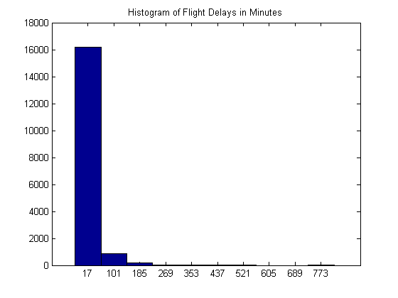
For example, using dot indexing you can plot a histogram of the departure delays (in minutes).
hist(FlightData.DEP_DELAY)
title('Histogram of Flight Delays in Minutes')

You can also display the first 5 departure delays.
FlightData.DEP_DELAY(1:5)
ans =
    49
    -7
    -5
    -8
   -10
You can also extract data from one or more variables in the table using curly braces. Within the curly braces you can use numeric indexing or variable and row names. For example, you can extract the actual departure times and scheduled depature times for the first 5 flights.
SomeTimes = FlightData{1:5,{'DEP_TIME','CRS_DEP_TIME'}};
disp(SomeTimes)
        1149        1100
        1053        1100
        1055        1100
        1052        1100
        1050        1100
This is similar to indexing with cell arrays. However, unlike with cells, this concatenates the specified variables into a single array. Therefore, the data types of all the specified variables need to be compatible for concatenation.
Converting Data to Categorical Arrays
You can convert some of the variables in your table using categorical. Categorical arrays are more memory efficent than holding cell arrays of strings when you have repeated data. Categorical arrays store only one copy of each category name, reducing the amount of memory required to store the array. You can use whos to see the amount of memory you save by converting the data to a categorical array.
whos FlightData
  Name                Size              Bytes  Class    Attributes

  FlightData      17816x7             9007742  table
FlightData.ORIGIN = categorical(FlightData.ORIGIN);
FlightData.DEST = categorical(FlightData.DEST);
FlightData.CARRIER = categorical(FlightData.CARRIER);

whos FlightData
  Name                Size              Bytes  Class    Attributes

  FlightData      17816x7             2857264  table
Using categories, you can find all the distinct categories in your array. By default, categorical arrays do not define a definite order. If your data contains categories with a definite order, you can set the 'Ordinal' flag to true when creating your categorical array. The default the order will be alphabetical, but you can prescribe you own order instead.
categories(FlightData.CARRIER)
ans =
    '9E'
    'AA'
    'AS'
    'B6'
    'CO'
    'DL'
    'F9'
    'FL'
    'MQ'
    'OH'
    'UA'
    'US'
    'WN'
    'XE'
    'YV'
Categorical arrays are also faster and more convenient than cell arrays of strings for indexing and searching. By converting to categorical arrays, you can then mathematically compare sets of strings just like you would do with numeric values. You can use this functionality to create a new table containing only the flights that left from Boston.
Creating a New Table
You can create a new table from a section of an existing table using parentheses with numerical indexing, variable names, or row names. Since the flight origin is now a categorical array, you can use logical indexing to find all flights that left from Boston.
idxBoston = FlightData.ORIGIN == 'BOS' ;
BostonFlights = FlightData(idxBoston,:);

height(FlightData)
height(BostonFlights)
ans =
       17816
ans =
        8904
Adding/Removing Variables
You can also modify your table by adding and removing variables and rows. All variables in a table must have the same number of rows, but they can be of different widths.
Let's add a new variable (DATE) to represent the serial date number for the various flight dates.
BostonFlights.DATE = datenum(BostonFlights.FL_DATE);
The origin now has all BOS values and you are not going to use destination information right now, so those variables can be removed. HOUR can also be calculated, as well as a LATE variable which indicates if the flight was 15 minutes late or more.
BostonFlights.ORIGIN = [];
BostonFlights.DEST = [];
BostonFlights.FL_DATE = [];

BostonFlights.HOUR = floor(BostonFlights.CRS_DEP_TIME./100);
BostonFlights{:,'LATE'} = BostonFlights.DEP_DELAY > 15;
Removing Missing Data
Tables have supported functions for finding and standardizing missing data. In this case, you can find any missing data using ismissing and remove it. You can use height, which gives you the number of table rows, to see how many flights were removed from the table. We exploit logical indexing to get only the flights that have no missing data.
height(BostonFlights)
ans =
        8904
TF = any(ismissing(BostonFlights),2);
BostonFlights = BostonFlights(~TF,:);
height(BostonFlights)
ans =
        8640
Summarizing a Table
You can then see descriptive statistics for each variable in this new table by using summary.
summary(BostonFlights)
Variables:
    CARRIER: 8640x1 categorical
        Values:
            9E      85
            AA     913
            AS      55
            B6    1726
            CO     321
            DL    1215
            F9      26
            FL     536
            MQ     751
            OH     341
            UA     643
            US    1494
            WN     384
            XE      93
            YV      57
    CRS_DEP_TIME: 8640x1 double
        Values:
            min        500
            median    1215
            max       2359
    DEP_TIME: 8640x1 double
        Values:
            min          2
            median    1224
            max       2400
    DEP_DELAY: 8640x1 double
        Values:
            min       -25
            median     -3
            max       419
    DATE: 8640x1 double
        Values:
            min       7.3414e+05
            median    7.3415e+05
            max       7.3417e+05
    HOUR: 8640x1 double
        Values:
            min        5
            median    12
            max       23
    LATE: 8640x1 logical
        Values:
            true     1471
            false    7169
Sorting Data
There are additional functions to sort tables, apply functions to table variables, and merge tables together. For example, you can sort your BostonFlights by departure delay.
BostonFlights = sortrows(BostonFlights,'DEP_DELAY','descend');
BostonFlights(1:10,:)
ans =
    CARRIER    CRS_DEP_TIME    DEP_TIME    DEP_DELAY       DATE       HOUR
    _______    ____________    ________    _________    __________    ____
    DL         1830             129        419          7.3416e+05    18
    DL         1850             111        381          7.3414e+05    18
    CO         1755              10        375          7.3414e+05    17
    AA         1710            2323        373          7.3416e+05    17
    DL          630            1240        370          7.3416e+05     6
    FL         1400            1951        351          7.3414e+05    14
    FL         1741            2330        349          7.3414e+05    17
    UA         1906              22        316          7.3414e+05    19
    AA          840            1355        315          7.3416e+05     8
    AA          905            1420        315          7.3414e+05     9

    LATE
    _____
    true
    true
    true
    true
    true
    true
    true
    true
    true
    true
Applying Functions to Table Variables
You can apply functions to work with table variables, with varfun.
varfun has optional additional calling inputs such as 'InputVariables' and 'GroupingVariables'. 'InputVariables' lets you specific which variables you want to operate on instead of operating on all the variables in your table. 'GroupingVariables' let you define groups of rows on which to operate. varfun would then apply your function to each group of rows within each of the variables of your table, rather than to each entire variable.
You can use varfun to calculate the mean delay for all flights and the fraction of late flights for a given hour on a given day. The default output of varfun is a table.
ByHour = varfun(@mean, BostonFlights, ...
    'InputVariables', {'DEP_DELAY', 'LATE'},...
    'GroupingVariables',{'DATE','HOUR'});

disp(ByHour(1:5,:))
                   DATE       HOUR    GroupCount    mean_DEP_DELAY    mean_LATE
                __________    ____    __________    ______________    _________
    734139_5    7.3414e+05    5        5               3.8                  0
    734139_6    7.3414e+05    6       19            10.579            0.31579
    734139_7    7.3414e+05    7       18            6.7778            0.11111
    734139_8    7.3414e+05    8       21            8.8571            0.33333
    734139_9    7.3414e+05    9       17            5.0588            0.23529
Joining (Merging) Tables
Weather might have an important role in determining if a flight is delayed. For a given hour, you might want to know both the delayed flight information and the weather at the airport. So, you can start by reading in another table containing weather data for Boston Logan Airport. Then, you can merge that table with the existing ByHour table.
Since there are a lot of variables in this file, you can specify the input format when using readtable. This allows you to use * to skip variables that you aren't interested in loading into the table. For more information about specifying formating strings, see here in the documentation. Since this data uses 'M' to represent missing data, you can use 'TreatAsEmpty' to replace any instances of 'M' with the standard missing value indicator (NaN for numeric values).
FormatStr = ['%*s%s%f' repmat('%*s',1,9) '%f' repmat('%*s',1,7) '%f',...
             repmat('%*s',1,3),'%f', repmat('%*s',1,18)];

WeatherData = readtable('BostonWeather.txt','HeaderLines',6,...
                        'Format',FormatStr,'TreatAsEmpty','M');

WeatherData.Properties.VariableNames
ans =
    'Date'    'Time'    'DryBulbCelsius'    'DewPointCelsius'    'WindSpeed'
WeatherData contains the date, time, dew point and dry bulb temperature in Celsius, and wind speed. Let's convert DATE to a serial date number and round to the hour for the time measurement.
WeatherData.DATE = datenum(WeatherData.Date,'yyyymmdd');
WeatherData.Date = [];
WeatherData.HOUR = floor(WeatherData.Time/100);
Since there are multiple weather measurements per hour, you can average the data by hour using varfun.
ByHourWeather = varfun(@mean, WeatherData, ...
    'InputVariables', {'DryBulbCelsius','DewPointCelsius','WindSpeed'},...
    'GroupingVariables',{'DATE','HOUR'});
Now, you can merge the two tables using join which matches rows using key variables (columns) common to both tables. join keeps all the variables from the first input table and appends the corresponding variables from the second input table. The table that join creates will use the key variable values as the row names. In this case, that means the row names will represent the date and hour data.
AllData = join(ByHour,ByHourWeather,'Keys',{'DATE','HOUR'});
Plotting Data From the Final Table
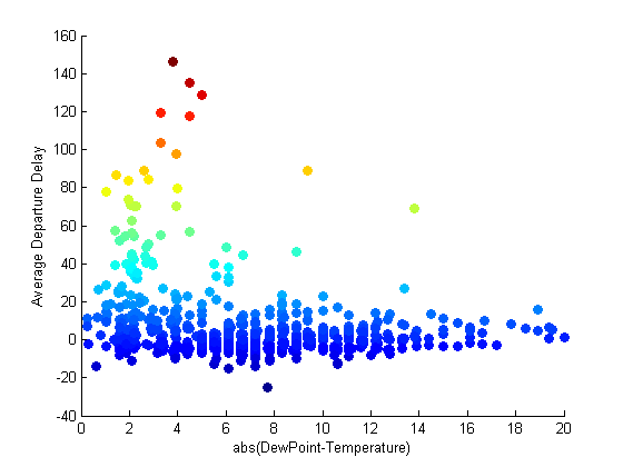
Let's now plot this final data set to get an idea of the effect of weather on the flight delays.
AllData.TDIFF =  ...
    abs(AllData.mean_DewPointCelsius - AllData.mean_DryBulbCelsius);

scatter(AllData.TDIFF, AllData.mean_DEP_DELAY,...
    [], AllData.mean_DEP_DELAY,'filled');
xlabel('abs(DewPoint-Temperature)')
ylabel('Average Departure Delay')

scatter3( AllData.HOUR,AllData.TDIFF,AllData.mean_DEP_DELAY,...
    [],AllData.mean_DEP_DELAY,'filled');
xlabel('Hour of Flight')
ylabel('abs(DewPoint-Temperature)')
zlabel('Average Departure Delay')

Qualitatively it looks having a temperature near the dew point (greater change of precipitation) effects the departure time. There are other factors at work as well, but it is nice to know that our intuition (flights later in the day and when it is cold and snowing might have a greater chance to be delayed) seems to work with the data.
Your Thoughts?
Can you see yourself using tables and categorical arrays? Let us know what you think or if you have any questions by leaving a comment here.
- カテゴリ:
- Data types,
- New Feature


コメント
コメントを残すには、ここ をクリックして MathWorks アカウントにサインインするか新しい MathWorks アカウントを作成します。