New Ways to Arrange and Plot Data in Tables
Today I'd like to introduce a guest blogger, Stephen Doe, who works for the MATLAB Documentation team here at MathWorks. In today's post, Stephen shows us new functions for displaying, arranging, and plotting data in tables and timetables.
Contents
Tables, Then and Now
In R2013b, MATLAB® introduced the table data type, as a convenient container for column-oriented data. And in R2016b, MATLAB introduced the timetable data type, which is a table that has timestamped rows.
From the beginning, these data types offered advantages over cell arrays and structures. But over the course of several releases, the table and graphics development teams have added many new functions for tables and timetables. These functions add convenient ways to display and arrange tabular data. Also, they offer new ways to make plots or charts directly from tables, without the intermediate step of peeling out variables. As of R2018b, MATLAB boasts many new functions to help you make more effective use of tables and timetables.
Read Table and Display First Few Rows
To begin, I will use the readtable function to read data from a sample file that ships with MATLAB. The file outages.csv contains simulated data for electric power outages over a period of 12 years in the United States. The call to readtable returns a table, T, with six variables and 1468 rows, so I will suppress the output using a semicolon.
T = readtable('outages.csv');
One typical way to examine the data in a large table is to display the first few rows of the table. You can use indexing to access a subset of rows (and/or a subset of variables, for that matter). For example, this syntax returns the first three rows of T.
T(1:3,:)
ans =
  3×6 table
      Region          OutageTime        Loss     Customers     RestorationTime         Cause
    ___________    ________________    ______    __________    ________________    ______________
    'SouthWest'    2002-02-01 12:18    458.98    1.8202e+06    2002-02-07 16:50    'winter storm'
    'SouthEast'    2003-01-23 00:49    530.14    2.1204e+05                 NaT    'winter storm'
    'SouthEast'    2003-02-07 21:15     289.4    1.4294e+05    2003-02-17 08:14    'winter storm'
I have a confession to make: I have written many table examples, using that syntax. And occasionally, I still catch myself starting with code like T(3,:), which accesses only one row.
Happily, in R2016b we added the head function to return the top rows of a table. Here's the call to return the first three rows using the head function.
head(T,3)
ans =
  3×6 table
      Region          OutageTime        Loss     Customers     RestorationTime         Cause
    ___________    ________________    ______    __________    ________________    ______________
    'SouthWest'    2002-02-01 12:18    458.98    1.8202e+06    2002-02-07 16:50    'winter storm'
    'SouthEast'    2003-01-23 00:49    530.14    2.1204e+05                 NaT    'winter storm'
    'SouthEast'    2003-02-07 21:15     289.4    1.4294e+05    2003-02-17 08:14    'winter storm'
Similarly, tail returns the bottom rows of a table. (If you do not specify the number of rows, then head and tail return eight rows.)
Move, Add, and Delete Table Variables
After examining your table, you might find that you want to organize your table by moving related variables next to each other. For example, in T you might want to move Region and Cause so that they are together.
One way to move table variables is by indexing. But if you use indexing and want to keep all the variables, then you must specify them all in order, as shown in this syntax.
T = T(:,{'OutageTime','Loss','Customers','RestorationTime','Region','Cause'})
You also can use numeric indices. While more compact, this syntax is less readable.
T = T(:,[2:5 1 6])
When your table has many variables, it is awkward to move variables using indexing. Starting in R2018a, you can use the movevars function instead. Using movevars, you only have to specify the variables of interest. Move the Region variable so it is before Cause.
T = movevars(T,'Region','Before','Cause');
head(T,3)
ans =
  3×6 table
       OutageTime        Loss     Customers     RestorationTime       Region           Cause
    ________________    ______    __________    ________________    ___________    ______________
    2002-02-01 12:18    458.98    1.8202e+06    2002-02-07 16:50    'SouthWest'    'winter storm'
    2003-01-23 00:49    530.14    2.1204e+05                 NaT    'SouthEast'    'winter storm'
    2003-02-07 21:15     289.4    1.4294e+05    2003-02-17 08:14    'SouthEast'    'winter storm'
It is also likely that you want to add data to your table. For example, let's calculate the duration of the power outages in T. Specify the format to display the duration in days.
OutageDuration = T.RestorationTime - T.OutageTime;
OutageDuration.Format = 'dd:hh:mm:ss';
It is easy to add OutageDuration to the end of a table using dot notation.
T.OutageDuration = OutageDuration;
However, you might want to add it at another location in T. In R2018a, you can use the addvars function. Add OutageDuration so that it is after OutageTime.
T = addvars(T,OutageDuration,'After','OutageTime');
head(T,3)
ans =
  3×7 table
       OutageTime       OutageDuration     Loss     Customers     RestorationTime       Region           Cause
    ________________    ______________    ______    __________    ________________    ___________    ______________
    2002-02-01 12:18     06:04:32:00      458.98    1.8202e+06    2002-02-07 16:50    'SouthWest'    'winter storm'
    2003-01-23 00:49             NaN      530.14    2.1204e+05                 NaT    'SouthEast'    'winter storm'
    2003-02-07 21:15     09:10:59:00       289.4    1.4294e+05    2003-02-17 08:14    'SouthEast'    'winter storm'
Now, let's remove RestorationTime. You can easily remove variables using dot notation and an empty array.
T.RestorationTime = [];
However, in R2018a there is also a function to remove table variables. To remove RestorationTime, use the removevars function.
T = removevars(T,'RestorationTime');
head(T,3)
ans =
  3×6 table
       OutageTime       OutageDuration     Loss     Customers       Region           Cause
    ________________    ______________    ______    __________    ___________    ______________
    2002-02-01 12:18     06:04:32:00      458.98    1.8202e+06    'SouthWest'    'winter storm'
    2003-01-23 00:49             NaN      530.14    2.1204e+05    'SouthEast'    'winter storm'
    2003-02-07 21:15     09:10:59:00       289.4    1.4294e+05    'SouthEast'    'winter storm'
Convert to Timetable
If your table contains dates and times in a datetime array, you can easily convert it to a timetable using the table2timetable function. In this example, table2timetable converts the values in OutageTime to row times. Row times are time stamps that label the rows of a timetable.
TT = table2timetable(T);
head(TT,3)
ans =
  3×5 timetable
       OutageTime       OutageDuration     Loss     Customers       Region           Cause
    ________________    ______________    ______    __________    ___________    ______________
    2002-02-01 12:18     06:04:32:00      458.98    1.8202e+06    'SouthWest'    'winter storm'
    2003-01-23 00:49             NaN      530.14    2.1204e+05    'SouthEast'    'winter storm'
    2003-02-07 21:15     09:10:59:00       289.4    1.4294e+05    'SouthEast'    'winter storm'
When you display a timetable, it looks very similar to a table. One important difference is that a timetable has fewer variables than you might expect by glancing at the display. TT has five variables, not six. The vector of row times, OutageTime, is not considered a timetable variable, since its values label the rows. However, you can still access the row times using dot notation, as in T.OutageTime. You can use the vector of row times as an input argument to a function. For example, you can use it as the x-axis of a plot.
The row times of a timetable do not have to be ordered. If you want to be sure that the rows of a timetable are sorted by the row times, use the sortrows function.
TT = sortrows(TT);
head(TT,3)
ans =
  3×5 timetable
       OutageTime       OutageDuration     Loss     Customers       Region           Cause
    ________________    ______________    ______    __________    ___________    ______________
    2002-02-01 12:18     06:04:32:00      458.98    1.8202e+06    'SouthWest'    'winter storm'
    2002-03-05 17:53     04:20:48:00      96.563    2.8666e+05    'MidWest'      'wind'
    2002-03-16 06:18     02:17:05:00      186.44    2.1275e+05    'MidWest'      'severe storm'
Make Stacked Plot of Variables
Now I will show you why I converted T to a timetable. Starting in R2018b, you can plot the variables of a table or timetable in a stacked plot. In a stacked plot, the variables are plotted in separate y-axes, but using a common x-axis. And if you make a stacked plot from a timetable, the x-values are the row times.
To plot the variables of TT, use the stackedplot function. The function plots variables that can be plotted (such as numeric, datetime, and categorical arrays) and ignores variables that cannot be plotted. stackedplot also returns properties of the stacked plot as an object that allows customization of the stacked plot.
s = stackedplot(TT)
s =
  StackedLineChart with properties:

         SourceTable: [1468×5 timetable]
    DisplayVariables: {'OutageDuration'  'Loss'  'Customers'}
               Color: [0 0.4470 0.7410]
           LineStyle: '-'
           LineWidth: 0.5000
              Marker: 'none'
          MarkerSize: 6

  Use GET to show all properties

One thing you can tell right away from this plot is that there must be a few timetable rows with bad data. There is one point for a power outage that supposedly lasted for over 9,000 days (or 24 years), which would mean it ended some time in the 2040s.
Convert Variables in Place
The stackedplot function ignored the Region and Cause variables, because these variables are cell arrays of character vectors. You might want to convert these variables to a different, and more useful, data type. While you can convert variables one at a time, there is now a more convenient way to convert all table variables of a specified data type.
Starting in R2018b, you can convert table variables in place using the convertvars function. For example, identify all the cell arrays of character vectors in TT (using iscellstr) and convert them to categorical arrays. Now Region and Cause contain discrete values assigned to categories. Categorical values are displayed without any quotation marks.
TT = convertvars(TT,@iscellstr,'categorical');
head(TT,3)
ans =
  3×5 timetable
       OutageTime       OutageDuration     Loss     Customers      Region         Cause
    ________________    ______________    ______    __________    _________    ____________
    2002-02-01 12:18     06:04:32:00      458.98    1.8202e+06    SouthWest    winter storm
    2002-03-05 17:53     04:20:48:00      96.563    2.8666e+05    MidWest      wind
    2002-03-16 06:18     02:17:05:00      186.44    2.1275e+05    MidWest      severe storm
Plots of Discrete Data
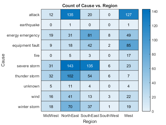
If your table or timetable has variables with values that belong to a finite set of discrete categories, then there are other interesting plots that you can make. Starting in R2017a, you can make a heat map of any two variables that contain discrete values using the heatmap function. For example, make a heat map of the Region and Cause variables to visualize where and why outages occur. Again, heatmap returns an object so you can customize the plot.
h = heatmap(TT,'Region','Cause')
h =
  HeatmapChart (Count of Cause vs. Region) with properties:

      SourceTable: [1468×5 timetable]
        XVariable: 'Region'
        YVariable: 'Cause'
    ColorVariable: ''
      ColorMethod: 'count'

  Use GET to show all properties

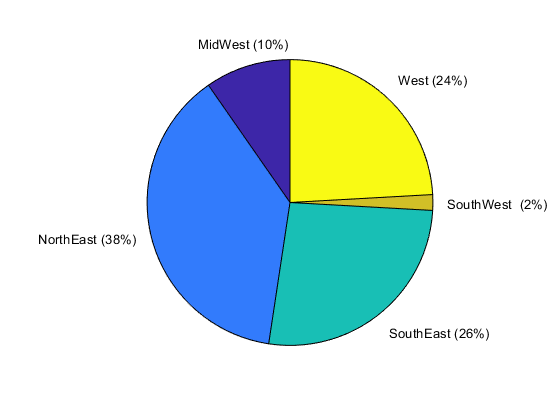
You also can make a pie chart of any categorical variable (as of R2014b), using the pie function. However, you cannot call pie on a table. So, to make a pie chart of the power outages by region, use dot notation to access the Region variable.
pie(TT.Region)

Other Functions to Rearrange or Join Tables
MATLAB also has other functions to reorganize variables in more complex ways, and to join tables. I won't show them all in action, but I will describe some of them briefly. All these functions work with both tables and timetables.
R2018a includes functions to:
- Reorient rows to become variables (rows2vars)
- Invert a nested table-in-table (inner2outer)
And from the original release of tables in R2013b, there are functions to:
Tabled for Discussion
Let's table discussion of these new functions for now. But we are eager to hear about your reactions to them. Do they help you make more effective use of tables and timetables? Please let us know here.
- Category:
- Data types,
- New Feature


Comments
To leave a comment, please click here to sign in to your MathWorks Account or create a new one.