Election Poll Analysis in MATLAB

This is a mid-term election year here in the United States, and today's guest blogger, Toshi Takeuchi, invites you to try election poll analysis with MATLAB for fun.

Contents

Why election polls?

Availability of abundant data, coupled with a very impressive success of a political outsider, Nate Silver, who made correct calls in the last two presidential elections, turned election poll analysis one of a fertile playgrounds for hobbyists to apply their data analytics skills for fun.

In this post, I would like to share an example of such analysis using a recent outcome of the special congressional election in Florida, along with a simple example of getting election poll data from Pollster website in JSON format and automating the data pull process with object oriented programming.

Does national politics affect local election?

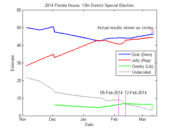
There was a race in Florida recently that was supposedly a test case for how Obama’s healthcare law impacts the mid-term election. Or was it?

What you can see in this plot is that the number of undecided voters suddenly dropped, and both Sink (D) and Jolly (R) benefited from it, but larger percentage of those voters actually ended up voting for Jolly, rather than Sink. This rapid shift happened around Feb 5 – 12. What I expected was a smoother decline of undecided voters over time, perhaps more accelerated toward the election day.

Could this have been caused by national politics?

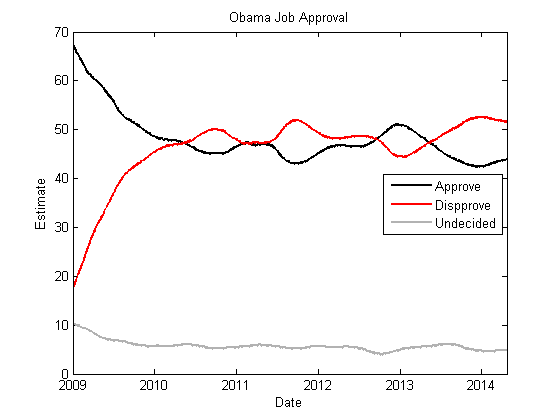
If you believe the pundits, then national issues like the healthcare law affects the local politics. Let’s use Obama’s job approval rating as a proxy to check it out.

As you can see in the plot, Obama’s national poll was actually going up towards the end of this election. This should have benefited Sink.

All politics is perhaps local

Actually, it is more important to see the local trend rather than the national trend. So use the polls from Florida alone to see the local Obama Job Approval trend.

Obama's Job Approval was recovering at the national level, but his approval was actually going down in Florida during this election. I am wondering what was happening around the time that the undecideds suddenly decided in the beginning of February. But can you really say this was the test of Obamacare?

National news headlines around that time:

Let me know if you have good data sources to test this claim. In my opinion, Obamacare alone doesn't seem to fully explain this rapid shift.

MATLAB example with Pollster API and JSONlab

Now I would like to address the programming aspect of this post. Pollster API provides convenient access to the data from election polls. There are other websites that aggregate election polls; this API was the easiest to use. JSON is a popular format for web services like this, and you can install an appropriate library from the FileExchange to process it. My favorite is JSONlab by Qianqian Fang.

Let’s start out with an simple example of getting data for Obama Job Approval Ratings.

baseUrl='http://elections.huffingtonpost.com/pollster/api/charts';
slug = 'obama-job-approval';
respFormat = 'json';
fullUrl = sprintf('%s/%s.%s',baseUrl,slug,respFormat);

% add jsonlab to the search path
addpath jsonlab;
% get the poll data
data=loadjson(urlread(fullUrl));

Convert the data into a table

JSON stores data in a nested tree structure like XML, so we need to convert it into a table in order to use the data in MATLAB. table is a new feature introduced in R2013b that I like quite a lot.

% initialize variables
estimates=data.estimates_by_date;
date = zeros(length(estimates),1);
approve = zeros(length(estimates),1);
disapprove = zeros(length(estimates),1);
undecided = zeros(length(estimates),1);

% loop over JSON tree
for i = 1:length(estimates)
    date(i) = datenum(estimates{i}.date);
    for j = 1:length(estimates{i}.estimates)
        if strcmpi('approve',estimates{i}.estimates{j}.choice)
            approve(i) = estimates{i}.estimates{j}.value;
        elseif strcmpi('disapprove',estimates{i}.estimates{j}.choice)
            disapprove(i) = estimates{i}.estimates{j}.value;
        else
            undecided(i) = estimates{i}.estimates{j}.value;
        end
    end
end

% consolidate the data into a table
estimates = table(date,approve,disapprove,undecided);
disp(estimates(1:5,:))

       date       approve    disapprove    undecided
    __________    _______    __________    _________
    7.3571e+05      44       51.5            0      
    7.3571e+05      44       51.6          4.8      
    7.3571e+05    43.9       51.6            0      
     7.357e+05    43.9       51.6          4.8      
     7.357e+05    43.9       51.6          4.8      

Remove missing values

Real data is never perfect, so we need to check for missing values and remove affected rows.

% get the indices of zero values
isMissing = table2array(estimates) == 0;
% get the count of missing values by variable
disp('number of missing values by variable')
disp(array2table(sum(isMissing),'VariableNames',estimates.Properties.VariableNames));
obamaDecided = estimates(~(isMissing(:,2) | isMissing(:,3)),1:3);
obamaUndecided = estimates(~isMissing(:,4),[1 4]);

number of missing values by variable
    date    approve    disapprove    undecided
    ____    _______    __________    _________
    0       1          1             205      

Plotting Obama Job Approval

In the final step, let's validate the data processing so far by plotting the data and compare it to the chart on Pollster website.

figure
plot(obamaDecided.date,obamaDecided.approve,'k-','LineWidth',2)
hold on
plot(obamaDecided.date,obamaDecided.disapprove,'r-','LineWidth',2)
h = plot(obamaUndecided.date,obamaUndecided.undecided,'b-','LineWidth',2);
set(h, 'color', [0.7 0.7 0.7])
datetick
xlabel('Date')
ylabel('Estimate')
legend('Approve','Dispprove','Undecided','Location','East')
title(data.title)
xlim([datenum('2009-01-01') Inf])
hold off

Automate the process with object oriented programming

As you can see, this is an iterative process, so it is a good idea to automate some of the steps. Let’s use object oriented programming to facilitate the data pull using a custom class called myPollster. This way, all the processed data is encapsulated in the object itself, and you don’t run into namespace issues.

The myPollster class also provides a utility method to return the logical indices of missing values in the table.

% instantiate the object
FL13 = myPollster();
% specify the slug for the data pull
slug = '2014-florida-house-13th-district-special-election';
% call the API and store the result in the object.
FL13.getChartData(slug);
% check the result
disp(FL13.title)
disp(FL13.T(1:5,:))

% Check for missing values
disp('check which variable contains missing values...')
disp(array2table(sum(FL13.isMissing),'VariableNames',FL13.T.Properties.VariableNames))

2014 Florida House: 13th District Special Election
       Date       Sink    Jolly    Overby    Undecided
    __________    ____    _____    ______    _________
    7.3567e+05      46    44.3     6.4       3.3      
    7.3567e+05      46    44.3     6.4       3.3      
    7.3567e+05      46    44.3     6.4       3.4      
    7.3567e+05    45.9    44.3     6.4       3.4      
    7.3567e+05    45.9    44.3     6.4       3.4      
check which variable contains missing values...
    Date    Sink    Jolly    Overby    Undecided
    ____    ____    _____    ______    _________
    0       0       0        28        0        

Have I whetted your appetite?

Hopefully this simple example was sufficient to get you interested in trying it yourself. In this example, I simply took the smoothed trend lines provided by Pollster, but you could also get individual poll data and build more complex model to make some prediction yourself.

Toshi

Get the MATLAB code

Published with MATLAB® R2014a