Reading Big Data into MATLAB
Today I’d like to introduce guest blogger Sarah Wait Zaranek who works for the MATLAB Marketing team here at MathWorks. Sarah previously has written about a variety of topics. Mostly recently, she cowrote a post with me about the new webcam capabilities in MATLAB. Today, Sarah will be discussing datastore, one of the new big data capabilities introduced in MATLAB R2014b.
Contents
- About the Data
- What is a Datastore?
- Defining Our Input Data
- Creating the DataStore
- Preview the Data
- Select Data to Import
- Adjust Variable Format
- Read in First Chunk
- Example 1: Read Selected Columns of Data for Use in Memory
- Example 2: Filter Data Down to a Subset for Use in Memory
- Example 3: Perform Analysis on Chunks of Data and Combine the Results
- Extending the Use of Datastore
- Conclusion
About the Data
datastore is used for reading data that is too large to fit in memory. For this example, we will be reading in data from the vehicle census of Massachusetts. It is a catalog of information about vehicle registered from 2008 to 2011. The dataset contains information about individual cars registered including vehicle type, location where the vehicle is housed, rated MPG, and measured CO_2 emissions. You can learn more about the data and even download it yourself, here. I have renamed the files in the demo for clarity's sake, but this is where they came from originally.
What is a Datastore?
As mentioned, a datastore is an object useful for reading collections of data that are too large to fit in memory.
Defining Our Input Data
datastore can work with a single file or a collection of files. In this case, we will be reading from a single file. Our file does not include variable names at the top of the file. They are listed in separate header file as defined below.
% Define Data File and Header File
datafile = 'vehiclebig.csv';
headerfile = 'varnames.txt';

% Read in Variable Names
fileID = fopen(headerfile);
varnames = textscan(fileID,'%s');
varnames = varnames{:};
fclose(fileID);
Creating the DataStore
We can now create our datastore by giving the name of the data file as the import to the datastore function. We also specify our datastore not use the first row of our file as variable names. We will set those variable names explicitly using the names found in the 'varnames.txt' file.
ds = datastore(datafile,'ReadVariableNames',false);

% Set Variable Names
ds.VariableNames = varnames
ds =
  TabularTextDatastore with properties:

                      Files: {
                             'H:\Documents\LOREN\MyJob\Art of MATLAB\SarahZ\datastore\vehiclebig.csv'
                             }
          ReadVariableNames: false
              VariableNames: {'record_id', 'vin_id', 'plate_id' ... and 42 more}

  Text Format Properties:
             NumHeaderLines: 0
                  Delimiter: ','
               RowDelimiter: '\r\n'
             TreatAsMissing: ''
               MissingValue: NaN

  Advanced Text Format Properties:
            TextscanFormats: {'%f', '%f', '%f' ... and 42 more}
         ExponentCharacters: 'eEdD'
               CommentStyle: ''
                 Whitespace: ' \b\t'
    MultipleDelimitersAsOne: false

  Properties that control the table returned by preview, read, readall:
      SelectedVariableNames: {'record_id', 'vin_id', 'plate_id' ... and 42 more}
            SelectedFormats: {'%f', '%f', '%f' ... and 42 more}
                RowsPerRead: 20000
Note that we haven't read in our data yet. We have just provided an easy way to access it through ds, our datastore.
Preview the Data
A really nice thing about a datastore is that you can preview your data without having to load it all into memory. datastore reads the data into a table which is a data type in MATLAB designed to work well with tabular data.
data = preview(ds);
whos data

data(:,1:7) % Look at first 7 variables
  Name      Size            Bytes  Class    Attributes

  data      8x45            21426  table

ans =
    record_id    vin_id     plate_id       me_id       owner_type    start_odom     start_date
    _________    ______    __________    __________    __________    __________    ____________
     2           1         5.3466e+06    1.2801e+07    1               NaN         '2011-11-07'
     4           1         5.3466e+06    1.1499e+07    1               NaN         '2009-08-27'
     7           2         6.6148e+06    1.2801e+07    1               NaN         '2011-11-19'
     9           2         6.6148e+06    1.1499e+07    1               NaN         '2008-07-01'
    10           3         6.4173e+06    1.2801e+07    1               NaN         '2011-12-06'
     1           1         5.3466e+06             1    1             30490         '2009-09-01'
     3           1         5.3466e+06             2    1             55155         '2010-10-02'
     5           2         6.6148e+06             3    1                 5         '2008-07-02'
By default, datastore will read in every column of our dataset. datastore makes an educated guess for the appropriate format for each column (variable) of our data. We can, however, specify a subset of columns or different formats if we wish.
Select Data to Import
We can specify which variables (columns) by setting the SelectedVariableNames property of our datastore. In this case, we only want to bring in 5 columns out of the 45.
ds.SelectedVariableNames = {'model_year', 'veh_type', ...
    'curbwt','mpg_adj','hybrid'};

preview(ds)
ans =
    model_year    veh_type    curbwt    mpg_adj    hybrid
    __________    ________    ______    _______    ______
    2008          'Car'       3500      21.65      0
    2008          'Car'       3500      22.54      0
    2008          'SUV'       4500         16      0
    2008          'SUV'       4500         17      0
    2005          'Truck'     5000      13.29      0
    2008          'Car'       3500      22.09      0
    2008          'Car'       3500      21.65      0
    2008          'SUV'       4500      16.66      0
Adjust Variable Format
We can adjust the format of the data we wish to access by using the SelectedFormats property. We can specify to bring in the vehicle type as a categorical variable by using the %C specifier. You can learn more here about the benefits of using categorical arrays.
ds.SelectedFormats;
ds.SelectedFormats{2} = '%C'  % read  in as a categorical
ds =
  TabularTextDatastore with properties:

                      Files: {
                             'H:\Documents\LOREN\MyJob\Art of MATLAB\SarahZ\datastore\vehiclebig.csv'
                             }
          ReadVariableNames: false
              VariableNames: {'record_id', 'vin_id', 'plate_id' ... and 42 more}

  Text Format Properties:
             NumHeaderLines: 0
                  Delimiter: ','
               RowDelimiter: '\r\n'
             TreatAsMissing: ''
               MissingValue: NaN

  Advanced Text Format Properties:
            TextscanFormats: {'%*q', '%*q', '%*q' ... and 42 more}
         ExponentCharacters: 'eEdD'
               CommentStyle: ''
                 Whitespace: ' \b\t'
    MultipleDelimitersAsOne: false

  Properties that control the table returned by preview, read, readall:
      SelectedVariableNames: {'model_year', 'veh_type', 'curbwt' ... and 2 more}
            SelectedFormats: {'%f', '%C', '%f' ... and 2 more}
                RowsPerRead: 20000
Read in First Chunk
We can use the read function to read in a chunk of our data. By default, read reads in 20000 rows at a time. This value can be adjusted using the RowsPerRead property.
testdata = read(ds);
whos testdata
  Name              Size             Bytes  Class    Attributes

  testdata      20000x5             683152  table
After you read in a chunk, you can use the hasdata function to see if there is still additional data available to read from the datastore.
hasdata(ds)
ans =
     1
By using hasdata and read in a while loop with your datastore, you can read in your entire dataset a piece at a time. We will put in a counter just to track how many read operations took place in our loop.
counter = 0;

while hasdata(ds)
    % Read in Chunk
    dataChunk = read(ds);
    counter = counter + 1;
end

counter
counter =
   825
By using reset, we can reset our datastore and start reading at the beginning of the file.
reset(ds)
Now that we see how to get started using datastore, let's look at 3 different ways to use it to work with a dataset that does not entirely fit in the memory of your machine.
Example 1: Read Selected Columns of Data for Use in Memory
If you are interested in only processing certain columns of your text file and those columns can fit in memory, you can use datastore to bring in those particular columns from your text file. Then, you can work with that data directly in memory. In this example, we are only interested in the model year and vehicle type of the cars that were registered. We can use readall instead of read to import all the selected data instead of just a chunk of it at a time.
ds.SelectedVariableNames = {'model_year', 'veh_type'};

cardata = readall(ds);
whos cardata
  Name                Size                Bytes  Class    Attributes

  cardata      16145383x2             161456272  table
Now that you have the data read into MATLAB, you can work with it like you would normally work with your data in MATLAB. For this example, we will just use the new histogram function introduced in R2014b to look at the distribution of vehicle model years registered.
figure
histogram(cardata.model_year)
hold on
histogram(cardata.model_year(cardata.veh_type == 'Car'))
hold off

xlabel('Model Year')
legend({'all vehicles', 'only cars'},'Location','southwest')

Example 2: Filter Data Down to a Subset for Use in Memory
Another way to subset your data is to filter the data down a chunk at time. Using datastore you can read in a chunk of data and keep only data you need from that chunk. You then continue this process, chunk by chunk, until you reach the end of the file and have only the subset of the data you want to use.
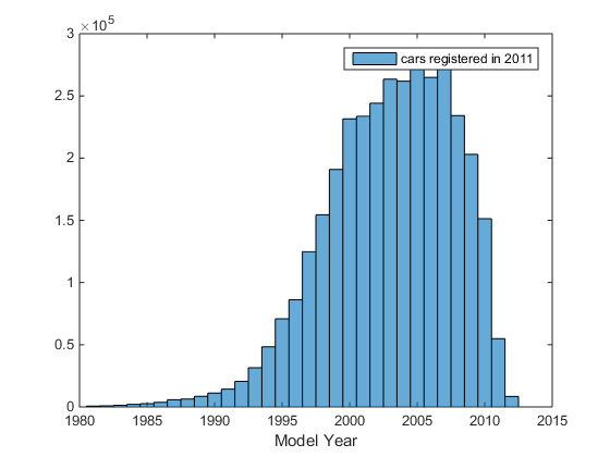
In this case, we want to extract a subset of data for cars that were registered in 2011. The new variables we are loading in (e.g., q1_2011), contain either a one or zero. Ones represent valid car registrations during that time. So we only save the rows which contain a valid registration sometime in 2011 and discard the rest.
reset(ds)
ds.SelectedVariableNames = {'model_year','veh_type',...
    'q1_2011','q2_2011','q3_2011','q4_2011'};

data2011 = table;

while hasdata(ds)

    % Read in Chunk
    dataChunk = read(ds);

    % Find if Valid During Any Quarter in 2011
    reg2011 = sum(dataChunk{:,3:end},2);

    % Extract Data to Keep (Cars Registered in 2011)
    idx = reg2011 >= 1 & dataChunk.veh_type == 'Car';

    % Save to Final Table
    data2011 = [data2011; dataChunk(idx,1:2)];

end

whos data2011

figure
histogram(data2011.model_year)
xlabel('Model Year')
legend({'cars registered in 2011'})
  Name                Size               Bytes  Class    Attributes

  data2011      3503434x2             35036782  table

Example 3: Perform Analysis on Chunks of Data and Combine the Results
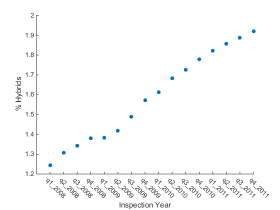
But what if we can't hold the subset of the data we are interested in analyzing in memory? We could instead process the data a section at a time and then combine intermediate results to get a final result. In this case, let's look at the % of hybrid cars registered every quarter (in terms of total cars registered). So, we compute a running total of the number of cars registered per quarter as well as the number of hybrids registered per quarter. Then, we calculate the final % when we have read through the entire dataset.
% Reset Datastore
reset(ds)

% Select Data to Import
quarterNames = varnames(end-15:end);
ds.SelectedVariableNames = [{'veh_type', 'hybrid'} quarterNames'];

% Read in Vehicle Type as a Categorical Variable
ds.SelectedFormats{1} = '%C';

totalCars = zeros(length(quarterNames),1);
totalHybrids = zeros(length(quarterNames),1);

while hasdata(ds)

    % Read in Chunk
    dataChunk = read(ds);

    for ii = 1:length(quarterNames) % Loop over car model years

    % Extract Data
    idx = dataChunk{:,quarterNames(ii)}== 1 & dataChunk.veh_type == 'Car';
    idxHy = idx & dataChunk.hybrid == 1;

    % Perform Calculation
    totalCarsChunk = sum(idx);
    totalHybridsChunk = sum(idxHy);

    % Save Result
    totalCars(ii) = totalCarsChunk + totalCars(ii);
    totalHybrids(ii) = totalHybridsChunk + totalHybrids(ii);

    end
end
percentHybrid = (totalHybrids./totalCars)*100;

figure
scatter(1:length(percentHybrid),percentHybrid,'filled')
xlabel('Inspection Year')
ylabel('% Hybrids')

% Label tick axes
ax = gca;
ax.TickLabelInterpreter = 'none';
ax.XTick = 1:length(quarterNames);
ax.XTickLabel = quarterNames;
ax.XTickLabelRotation = -45;

Extending the Use of Datastore
You can also use datastore as the first step to creating and running your own MapReduce algorithms in MATLAB. Perhaps this topic will be a blog post in the future.
Conclusion
Do you think you can use datastore with your big data? Let us know here.
 Cleve’s Corner: Cleve Moler on Mathematics and Computing
 The MATLAB Blog
 Guy on Simulink
 MATLAB Community
 Artificial Intelligence
 Developer Zone
 Stuart’s MATLAB Videos
 Behind the Headlines
 File Exchange Pick of the Week
 Hans on IoT
 Student Lounge
 MATLAB ユーザーコミュニティー
 Startups, Accelerators, & Entrepreneurs
 Autonomous Systems
 Quantitative Finance
 MATLAB Graphics and App Building


댓글
댓글을 남기려면 링크 를 클릭하여 MathWorks 계정에 로그인하거나 계정을 새로 만드십시오.