In 2016, we published this blog post simulating a pole vault jump. I decided to revisit this topic and demonstrate how I would simulate this using the latest features in Simulink. Pole Vault Model
Here is an illustration of what a pole vault jump looks like:
To simulate this event, we can divide the jump in three phases:
- Approach: During this phase the athlete tries to maximize his speed along the runway to achieve maximum kinetic energy
- Take off and swing up: The athlete positions the pole into the “box” to convert the kinetic energy into stored potential energy in the pole and swing up.
- Fly away: The vaulter releases the pole and falls back on the mat under the influence of gravity
In 2016, the way to model that was using a series of 3 If Action Subsystems. When switching from one phase to the next, we would transfer the states from one Subsystem to the next using the Integrator block state port and GoTo and From blocks. This semantic had multiple imitations. Let's see my preferred way to implement the same equations in MATLAB R2024a.
Simulink States inside Stateflow
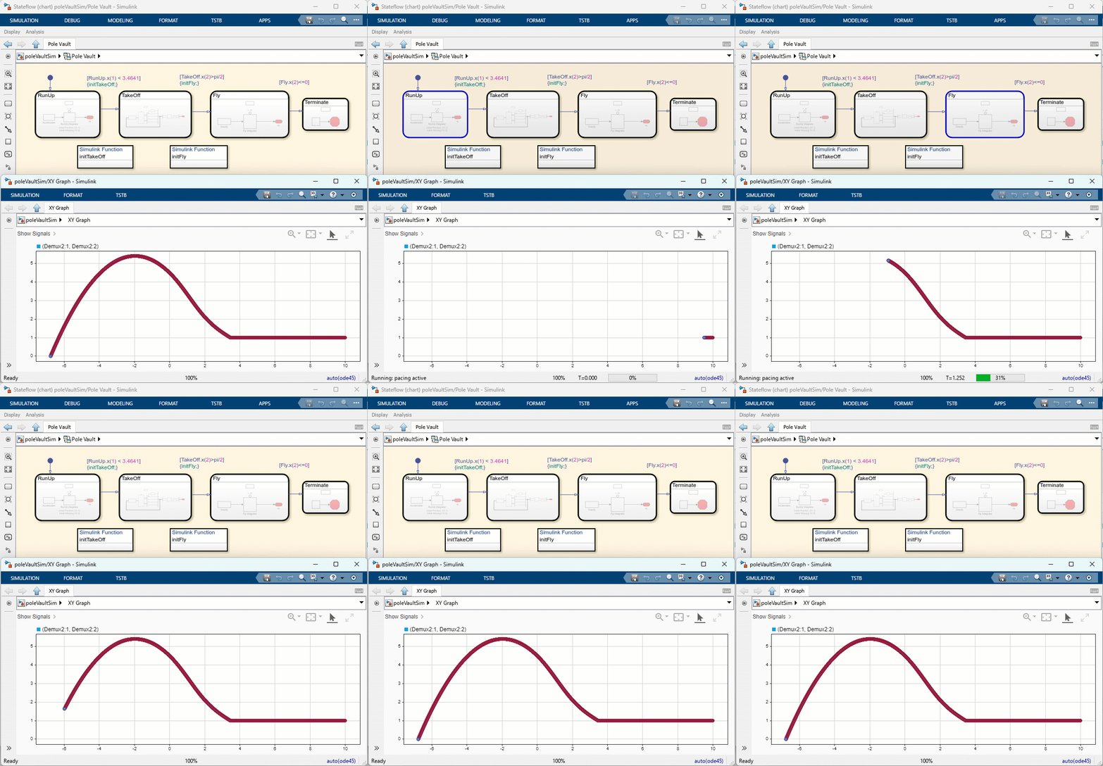
Here is what my new model looks like.
mdl = "poleVaultSim";
open_system(mdl);
Yes, this is correct, only one Stateflow Chart. Don't be fooled, the Simulink blocks are inside! During the Run Up phase, I integrate the motion of the athlete running at a constant speed. Compared to the 2016 implementation, I am able to use the Second Order Integrator instead of two Integrator blocks, because the Second Order Integrator does not have a state port option. During the Take Off, the motion of the athlete is computed in polar coordinate. This makes it simpler to solve the equations for the bending of the pole.
The important part to notice is what happens in the Simulink Functions. Using State Reader blocks, I can access the states of the Integrator blocks in the previous phase and compute the initial states of the next phase. I can then use State Writer blocks to initialize the Integrator blocks in the next phase. When simulating the model, we can follow the evolution of the simulation through the Stateflow animation and the newly revamped XY Graph block, which is just a pre-configured instance of the Record block. Design Study
Let's see the impact on the jump of two variables:
- The stiffness of the pole
- The initial angle of the pole for the take-off phase
For that, I create two multisim variables and combine them using simulink.multisim.Exhaustive.
mdl = "poleVaultSim";
k_var = simulink.multisim.Variable("k", linspace(0.1,10,5));
theta0_var = simulink.multisim.Variable("theta0", linspace(10,50,5));
MyCombination = simulink.multisim.Exhaustive([k_var, theta0_var]);
d = simulink.multisim.DesignStudy(mdl,MyCombination);
d.PostSimFcn = @(simOut, simIn) myPostSim(simOut,simIn);
out = parsim(d,'ShowProgress','off','UseFastRestart','on');
I also create a post-sim function where I do two things:
- I store the input variables in the SimulationOutput object
- I process the logged data to compute the maximum height and distance of the jump
Once the simulations complete, we can visualize results in multiple ways. Let's try a few things.
Let's begin by plotting all x-y timeseries:
figure;hold on;
for i = 1:length(out)
plot(out(i).logsout.get('x').Values.Data,out(i).logsout.get('y').Values.Data)
legendText{i} = ['k = ' num2str(out(i).k) ', theta0 = ' num2str(out(i).theta0)];
end
legend(legendText,'Location','northeastoutside');
Maybe a matrix of scatter plots would help visualize this data?
u = [[out.k]' [out.theta0]'];
y = [[out.maxHeight]' [out.distance]'];
figure;
or a 3d bar plot?
height = reshape([out.maxHeight],5,5);
figure
In the end, this seems pretty clear that the lower stiffness and initial angle result in the higher jump.
Now it's your turn
Don't miss the actual pole vault competition at the Paris Olympic:
How would you simulate the pole vault competition? Let us know in the comments below.


 Cleve’s Corner: Cleve Moler on Mathematics and Computing
 The MATLAB Blog
 Guy on Simulink
 MATLAB Community
 Artificial Intelligence
 Developer Zone
 Stuart’s MATLAB Videos
 Behind the Headlines
 File Exchange Pick of the Week
 Internet of Things
 Student Lounge
 MATLAB ユーザーコミュニティー
 Startups, Accelerators, & Entrepreneurs
 Autonomous Systems
 Quantitative Finance
 MATLAB Graphics and App Building
 Semiconductor Design and Verification


Comments
To leave a comment, please click here to sign in to your MathWorks Account or create a new one.