
Olympic 2016 – Pole Vault
For this second post in our Olympics series, I am happy to welcome guest blogger Amit Raj to describe how he simulated the pole vault competition.
Introduction
Track and field events are one of the most popular kinds of athletic sports in the Olympics. Pole vaulting is a track and field event where an athlete uses a long flexible pole as an aid to jump over a bar. Historically pole vaults were used to jump over canals and marshes. Pole vaulting has featured as an event in the Olympics since 1896.

Conservation of Energy
Vaulting is a prime example to demonstrate the conservation of energy principle. The athlete builds up kinetic energy and uses the pole to convert this into potential energy.
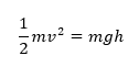
The current world record stands at 6.14 m set by Sergey Bubka. The record for fastest sprint is by Usain Bolt, at a little over 12 m/s. However, vaulters need to sprint with the weight of the pole. If we are reasonable and assume a sprint of 10m/s, that gives us a height of:
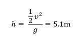
This is the change in height of center of mass. If we assume an initial height of center of mass at 1m we have a height of 6.102 which is pretty close to the world record.
Physics works... Yeah!
The phases
Although speed is important to determine the height, the technique of the vaulter also decides how effectively all the kinetic energy can be converted into potential energy. The conversion usually happens in multiple stages.
The generally accepted model for pole vaulting consist of the following phases:
- Approach: During this phase the athlete tries to maximize his speed along the runway to achieve maximum kinetic energy
- Plant and take off: The athlete positions the pole into the “box” to convert the kinetic energy into stored potential energy in the pole
- Swing up: The athlete moves the swing leg forward and tries to keep the pole bent longer to achieve an optimal position for the
release - Turn: The vaulter spins 180 towards the pole while extending the arm
- Fly away: The vaulter releases the pole and falls back on the mat under the influence of gravity
Let's now see how we can simulate that.
The Model
We model the above phases using three main stages – The run up, take off and release. In Simulink, each stage is a If Action Subsystem governed by its own set of dynamic equations. The challenge lies in switching between the different dynamics and still maintaining continuity.
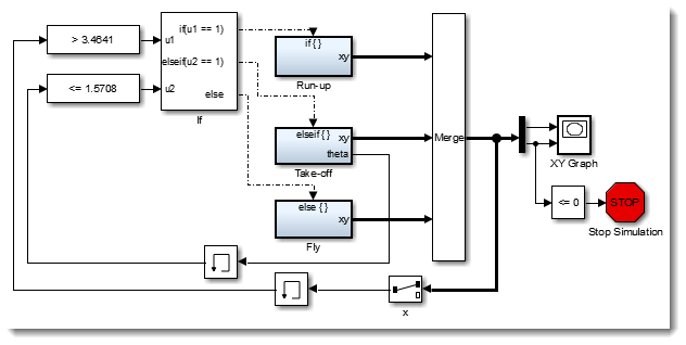
The first phase is quite simple, we just run at a constant speed of 10 m/s. The important thing to note here is the usage of the state port.
When the If condition changes from the running subsystem to the takeoff, the state ports of the Integrator blocks write to Goto blocks. In the Takeoff subsystem, we can then use From blocks to receive the final state of the run to initialize the takeoff subsystem.
In this case, the run was computed in a Cartesian coordinate system, but we decided to implement the takeoff in a polar coordinate system. Solving the equation for the bending of the pole is simpler in polar coordinates, where the integrated states are the length and angle of the pole.
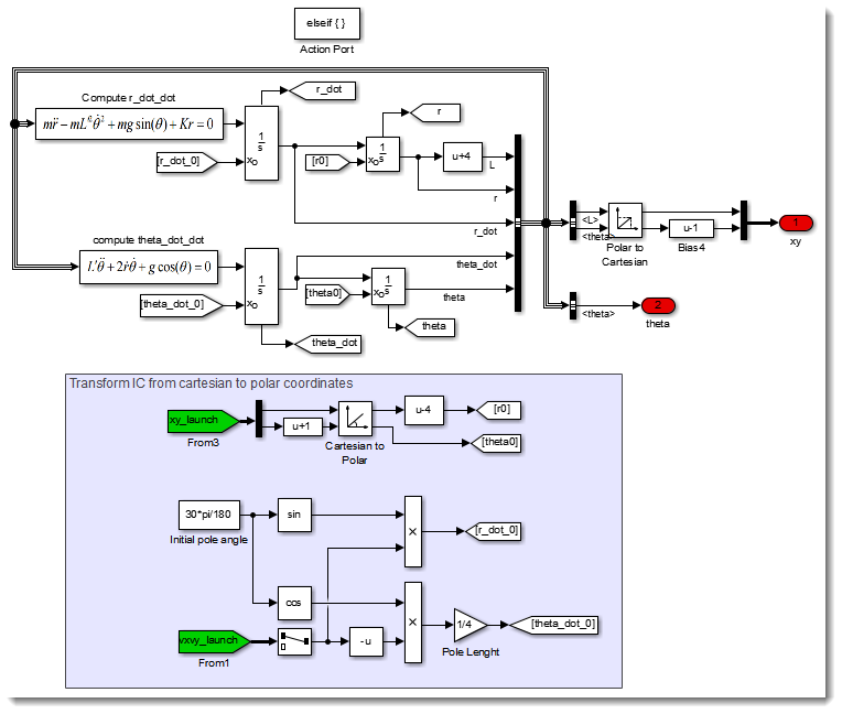
Once the pole reaches 90 degrees, it is time to let it go and switch to the flying phase.
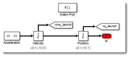
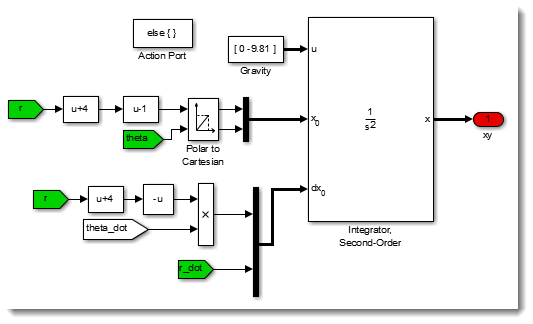
In a similar manner as the previous transition, we pass the final states through Goto and From blocks. In the flight subsystem, we convert back to Cartesian coordinates and let the gravity do the work.
Now it's your turn
Download the model here, and try different parameters to see what is the optimal configuration to win the pole vault competition at the Olympics.
- Category:
- Challenge,
- Fun,
- Guest Blogger,
- Modeling


Comments
To leave a comment, please click here to sign in to your MathWorks Account or create a new one.