Feret Diameter: Introduction

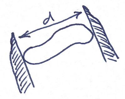
Posted by Steve Eddins, September 29, 2017

83 views (last 30 days) | 0 Likes | 8 comments

This is the first of a few blog posts about object measurements based on a concept called the Feret diameter, sometimes called the caliper diameter. The diagram below illustrates the concept. Place the object to be measured inside the jaws of a caliper, with the caliper oriented at a specified angle. Close the jaws tightly on the object while maintaining that angle. The distance between the jaws is the Feret diameter at that angle.

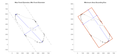
Eventually, we'll examine several related measurements (and algorithms for computing them), like these.

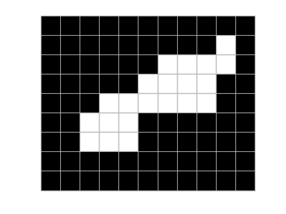
Today, though, I'm just going to play around with a very small binary image. (Note: the pixelgrid function is a utility that I wrote. It's at the bottom of this post.)

bw = [ ...
    0   0   0   0   0   0   0   0   0   0   0
    0   0   0   0   0   0   0   0   0   1   0
    0   0   0   0   0   0   1   1   1   1   0
    0   0   0   0   0   1   1   1   1   0   0
    0   0   0   1   1   1   1   1   1   0   0
    0   0   1   1   1   0   0   0   0   0   0
    0   0   1   1   1   0   0   0   0   0   0
    0   0   0   0   0   0   0   0   0   0   0
    0   0   0   0   0   0   0   0   0   0   0 ];


imshow(bw)
pixelgrid

I want to brute-force my to finding the two corners of the white blob that are farthest apart. Let's start by finding all the pixel corners. (I'll be using implicit expansion here, which works in R2016b or later.)

[y,x] = find(bw);
hold on
plot(x,y,'xb','MarkerSize',5)
corners = [x y] + cat(3,[.5 .5],[.5 -.5],[-.5 .5],[-.5 -.5]);
corners = permute(corners,[1 3 2]);
corners = reshape(corners,[],2);
corners = unique(corners,'rows');
plot(corners(:,1),corners(:,2),'sr','MarkerSize',5)
hold off

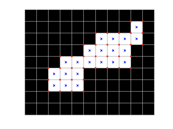
Well, let's get away from pure brute force just a little. We really only need to look at the points that are part of the convex hull of all the corner points.

hold on
k = convhull(corners);
hull_corners = corners(k,:);
plot(hull_corners(:,1),hull_corners(:,2),'r','LineWidth',3)
plot(hull_corners(:,1),hull_corners(:,2),'ro','MarkerSize',10,'MarkerFaceColor','r')
hold off

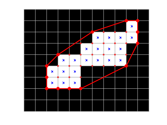
Now let's find which two points on the convex hull are farthest apart.

dx = hull_corners(:,1) - hull_corners(:,1)';
dy = hull_corners(:,2) - hull_corners(:,2)';
pairwise_dist = hypot(dx,dy);
[max_dist,j] = max(pairwise_dist(:));
[k1,k2] = ind2sub(size(pairwise_dist),j);

point1 = hull_corners(k1,:);
point2 = hull_corners(k2,:);
hold on
plot([point1(1) point2(1)],[point1(2) point2(2)],'-db','LineWidth',3,'MarkerFaceColor','b')
hold off

And the maximum distance is ...

max_dist

max_dist =

    10

(I thought I had made a mistake when I first saw this number come out to be an exact integer. But no, the answer is really 10.)

That's a pretty good start. I don't know exactly where I'll go with this topic next time. I'm making it up as I go.

function hout = pixelgrid(h)
%pixelgrid Superimpose a grid of pixel edges on an image
%   pixelgrid superimposes a grid of pixel edges on the image in the
%   current axes.
%
%   pixelgrid(h_ax) superimposes the grid on the image in the specified
%   axes.
%
%   pixelgrid(h_im) superimposes the grid on the specified image.
%
%   group = pixelgrid(___) returns an hggroup object that contains the two
%   lines that are used to draw the grid. One line is thick and darker, and
%   the other is thin and lighter. Using two contrasting lines in this way
%   guarantees that the grid will be visible regardless of pixel colors.
%
%   EXAMPLES
%
%   Superimpose pixel grid on color image. Zoom in.
%
%       rgb = imread('peppers.png');
%       imshow(rgb)
%       pixelgrid
%       axis([440 455 240 250])
%
%   Change the colors and line widths of the pixel grid.
%
%       rgb = imread('peppers.png');
%       imshow(rgb)
%       h = pixelgrid;
%       axis([440 455 240 250])
%       h.Children(1).Color = [178 223 138]/255;
%       h.Children(1).LineWidth = 2;
%       h.Children(2).Color = [31 120 180]/255;
%       h.Children(2).LineWidth = 4;
%
%   LIMITATIONS
%
%   This function is intended for use when looking at a zoomed-in image
%   region with a relatively small number of rows and columns. If you use
%   this function on a typical, full-size image without zooming in, the
%   image will not be visible under the grid lines.
%
%   This function attempts to determine if MATLAB is running with a high
%   DPI display. If so, then it displays the pixel grid using thinner
%   lines. However, the method for detecting a high DPI display on works on
%   a Mac when Java AWT is available.

%   Steve Eddins
%   Copyright The MathWorks, Inc. 2017

if nargin < 1
    him = findobj(gca,'type','image');
elseif strcmp(h.Type,'axes')
    him = findobj(h,'type','image');
elseif strcmp(h.Type,'image')
    him = h;
else
    error('Invalid graphics object.')
end

if isempty(him)
    error('Image not found.');
end

hax = ancestor(him,'axes');

xdata = him.XData;
ydata = him.YData;
[M,N,~] = size(him.CData);

if M > 1
    pixel_height = diff(ydata) / (M-1);
else
    % Special case. Assume unit height.
    pixel_height = 1;
end

if N > 1
    pixel_width = diff(xdata) / (N-1);
else
    % Special case. Assume unit width.
    pixel_width = 1;
end

y_top = ydata(1) - (pixel_height/2);
y_bottom = ydata(2) + (pixel_height/2);
y = linspace(y_top, y_bottom, M+1);

x_left = xdata(1) - (pixel_width/2);
x_right = xdata(2) + (pixel_width/2);
x = linspace(x_left, x_right, N+1);

% Construct xv1 and yv1 to draw all the vertical line segments. Separate
% the line segments by NaN to avoid drawing diagonal line segments from the
% bottom of one line to the top of the next line over.
xv1 = NaN(1,3*numel(x));
xv1(1:3:end) = x;
xv1(2:3:end) = x;
yv1 = repmat([y(1) y(end) NaN], 1, numel(x));

% Construct xv2 and yv2 to draw all the horizontal line segments.
yv2 = NaN(1,3*numel(y));
yv2(1:3:end) = y;
yv2(2:3:end) = y;
xv2 = repmat([x(1) x(end) NaN], 1, numel(y));

% Put all the vertices together so that they can be drawn with a single
% call to line().
xv = [xv1(:) ; xv2(:)];
yv = [yv1(:) ; yv2(:)];

hh = hggroup(hax);
dark_gray = [0.3 0.3 0.3];
light_gray = [0.8 0.8 0.8];

if isHighDPI
    bottom_line_width = 1.5;
    top_line_width = 0.5;
else
    bottom_line_width = 3;
    top_line_width = 1;
end

% When creating the lines, use AlignVertexCenters to avoid antialias
% effects that would cause some lines in the grid to appear brighter than
% others.
line(...
    'Parent',hh,...
    'XData',xv,...
    'YData',yv,...
    'LineWidth',bottom_line_width,...
    'Color',dark_gray,...
    'LineStyle','-',...
    'AlignVertexCenters','on');
line(...
    'Parent',hh,...
    'XData',xv,...
    'YData',yv,...
    'LineWidth',top_line_width,...
    'Color',light_gray,...
    'LineStyle','-',...
    'AlignVertexCenters','on');

% Only return an output if requested.
if nargout > 0
    hout = hh;
end

end

function tf = isHighDPI
% Returns true if running with a high DPI default display.
%
% LIMITATION: Only works on a Mac with Java AWT available. In other
% situations, this function always returns false.
tf = false;
if ismac
    if usejava('awt')
        sf = java.awt.GraphicsEnvironment.getLocalGraphicsEnvironment().getDefaultScreenDevice.getScaleFactor();
        tf = sf > 1;
    end
end
end