
Feret Diameters and Antipodal Vertices
Last time, I wrote about finding the maximum Feret diameter for an object in a binary image, ending up with this figure:

I had computed the convex hull of all the pixel corners, and then I computed the pairwise distance between every pair of convex hull vertices to find the maximum distance.
The procedure would work fine in many cases, but the time required to find the maximum distance this way grows with the square of the number of convex hull vertices. With modern digital image resolutions, it's not hard to imagine having thousands of vertices and therefore millions of pairwise distances to compute.
There is a procedure for reducing the number of vertex pairs we can consider. It is based on this theorem:
The diameter of a convex figure is the greatest distance between parallel lines of support. [Theorem 4,18, Preparata and Shamos, Computational Geometry, 1985]
A line of support for a polygon is a line that contains a vertex of the polygon, with the polygon lying entirely on one side of the line.
Let me show you a picture using the convex hull points from last time.
hull = [
    2.5000    5.5000
    3.5000    4.5000
    6.5000    2.5000
    9.5000    1.5000
   10.5000    1.5000
   10.5000    3.5000
    9.5000    5.5000
    5.5000    7.5000
    2.5000    7.5000
    2.5000    5.5000  ];

plot(hull(:,1),hull(:,2),'r','LineWidth',2)
hold on
plot(hull(:,1),hull(:,2),'r*')
hold off
axis equal
axis ij
axis([0 15 0 10])

for theta = -55:5:-35
    drawFullLine(gca,[9.5 5.5],theta,'Color',[.6 .6 .6]);
end
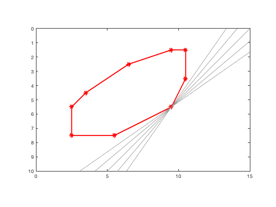
The plot above shows five different lines of support drawn through the (9.5,5.5) vertex. Now I'll add some of the lines of support through the (2.5,7.5) vertex.
for theta = 10:10:80
    drawFullLine(gca,[2.5 7.5],theta,'Color',[.6 .6 .6]);
end

You can see that there is no line of support for the (2.5,7.5) vertex that is parallel to a line of support for the (9.5,5.5) vertex. That rules out this pair of vertices for computing the maximum Feret diameter.
Now I'll draw lines of support for a different pair of vertices.
plot(hull(:,1),hull(:,2),'r','LineWidth',2)
hold on
plot(hull(:,1),hull(:,2),'r*')
hold off
axis equal
axis ij
axis([0 15 0 10])

drawFullLine(gca,[6.5 2.5],-30,'Color',[.6 .6 .6]);
drawFullLine(gca,[9.5 5.5],-30,'Color',[.6 .6 .6]);
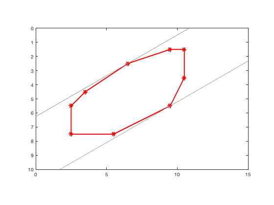
Because the vertices (6.5,2.5) and (9.5,5.5) have parallel lines of support, they are called antipodal vertices. There is an algorithm in the Preparata and Shamos book (referenced above) that finds all the antipodal vertices for a convex polygon. There's an implementation of the algorithm in a function at the bottom of this post. I'll use it to find all the antipodal pairs of the convex hull vertices.
pq = antipodalPairs(hull);
Important note: the algorithm in antipodalPairs assumes that its input is convex. Further, it assumes that the input does not contain any vertices that are on the straight line between the two adjacent vertices. To satisfy this condition, compute the convex hull using the call: k = convhull(P,'Simplify',true).
Now let's plot the line segments joining each antipodal pair.
plot(hull(:,1),hull(:,2),'r','LineWidth',2)
hold on
plot(hull(:,1),hull(:,2),'r*')
axis equal
axis ij
axis([0 15 0 10])

for k = 1:size(pq,1)
    x = [hull(pq(k,1),1) hull(pq(k,2),1)];
    y = [hull(pq(k,1),2) hull(pq(k,2),2)];
    plot(x,y,'Color',[.6 .6 .6]);
end
hold off
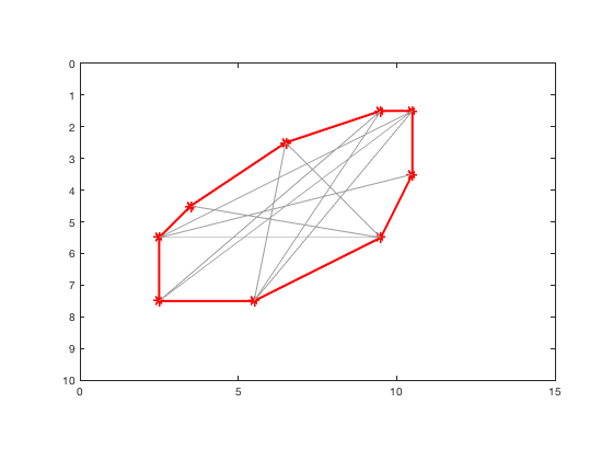
To find the maximum Feret diameter, we only have to check the distances of these 10 segments, instead of 10*9 = 90 line segments as before.
p1 = hull(pq(:,1),:);
p2 = hull(pq(:,2),:);
v = p1 - p2;
d = hypot(v(:,1),v(:,2));
[d_max,idx] = max(d);
p1_max = p1(idx,:);
p2_max = p2(idx,:);
hold on
plot([p1_max(1) p2_max(1)],[p1_max(2) p2_max(2)],'b','LineWidth',2)
hold off
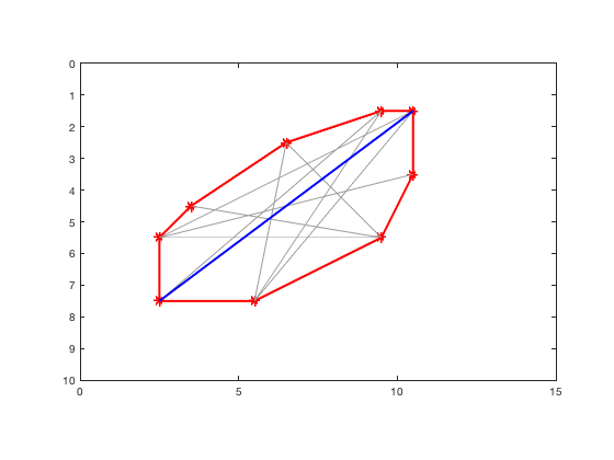
d_max
d_max =

    10
And there is the maximum Feret distance.
I am sure that, in many cases, it would be quicker to find the maximum distance by brute force comparison of all pairs off convex hull vertices. The computation of the antipodal pairs does take some time, after all. I have not done a performance study to investigate this question further. However, the antipodal pairs computation is useful for another measurement: the minimum Feret distance.
I will look at that next time.
End of post
Algorithm, visualization, and utility functions used by the code above
function h = drawFullLine(ax,point,angle_degrees,varargin)
%drawFullLine Draw a line that spans the entire plot
%
%    drawFullLine(ax,point,angle_degrees) draws a line in the
%    specified axes that goes through the specified point at the
%    specified angle (in degrees). The line is drawn to span the
%    entire plot.
%
%    drawFullLine(___,Name,Value) passes name-value parameter pairs
%    to the line function.

% Steve Eddins


limits = axis(ax);
width = abs(limits(2) - limits(1));
height = abs(limits(4) - limits(3));
d = 2*hypot(width,height);
x1 = point(1) - d*cosd(angle_degrees);
x2 = point(1) + d*cosd(angle_degrees);
y1 = point(2) - d*sind(angle_degrees);
y2 = point(2) + d*sind(angle_degrees);
h = line(ax,'XData',[x1 x2],'YData',[y1 y2],varargin{:});
end

function pq = antipodalPairs(S)
% antipodalPairs Antipodal vertex pairs of simple, convex polygon.
%
%   pq = antipodalPairs(S) computes the antipodal vertex pairs of a simple,
%   convex polygon. S is a Px2 matrix of (x,y) vertex coordinates for the
%   polygon. S must be simple and convex without repeated vertices. It is
%   not checked for satisfying these conditions. S can either be closed or
%   not. The output, pq, is an Mx2 matrix representing pairs of vertices in
%   S. The coordinates of the k-th antipodal pair are S(pq(k,1),:) and
%   S(pq(k,2),:).
%
%   TERMINOLOGY
%
%   For a convex polygon, an antipodal pair of vertices is one where you
%   can draw distinct lines of support through each vertex such that the
%   lines of support are parallel.
%
%   A line of support is a line that goes through a polygon vertex such
%   that the interior of the polygon lies entirely on one side of the line.
%
%   EXAMPLE
%
%     Compute antipodal vertices of a polygon and plot the corresponding
%     line segments.
%
%       x = [0 0 1 3 5 4 0];
%       y = [0 1 4 5 4 1 0];
%       S = [x' y'];
%       pq = antipodalPairs(S);
%
%       plot(S(:,1),S(:,2))
%       hold on
%       for k = 1:size(pq,1)
%           xk = [S(pq(k,1),1) S(pq(k,2),1)];
%           yk = [S(pq(k,1),2) S(pq(k,2),2)];
%           plot(xk,yk,'LineStyle','--','Marker','o','Color',[0.7 0.7 0.7])
%       end
%       hold off
%       axis equal
%
%   ALGORITHM NOTES
%
%   This function uses the "ANTIPODAL PAIRS" algorithm, Preparata and
%   Shamos, Computational Geometry: An Introduction, Springer-Verlag, 1985,
%   p. 174.

%   Steve Eddins


n = size(S,1);

if isequal(S(1,:),S(n,:))
    % The input polygon is closed. Remove the duplicate vertex from the
    % end.
    S(n,:) = [];
    n = n - 1;
end

% The algorithm assumes the input vertices are in counterclockwise order.
% If the vertices are in clockwise order, reverse the vertices.
clockwise = simplePolygonOrientation(S) < 0;
if clockwise
    S = flipud(S);
end

% The following variables, including the two anonymous functions, are set
% up to follow the notation in the pseudocode on page 174 of Preparata and
% Shamos. p and q are indices (1-based) that identify vertices of S. p0 and
% q0 identify starting vertices for the algorithm. area(i,j,k) is the area
% of the triangle with the corresponding vertices from S: S(i,:), S(j,:),
% and S(k,:). next(p) returns the index of the next vertex of S.
%
% The initialization of p0 is missing from the Preparata and Shamos text.
area = @(i,j,k) signedTriangleArea(S(i,:),S(j,:),S(k,:));
next = @(i) mod(i,n) + 1; % mod((i-1) + 1,n) + 1
p = n;
p0 = next(p);
q = next(p);

% The list of antipodal vertices will be built up in the vectors pp and qq.
pp = zeros(0,1);
qq = zeros(0,1);

% ANTIPODAL PAIRS step 3.
while (area(p,next(p),next(q)) > area(p,next(p),q))
    q = next(q);
end
q0 = q;    % Step 4.

while (q ~= p0)    % Step 5.
    p = next(p);   % Step 6.
    % Step 7. (p,q) is an antipodal pair.
    pp = [pp ; p];
    qq = [qq ; q];

    % Step 8.
    while (area(p,next(p),next(q)) > area(p,next(p),q))
        q = next(q);    % Step 9.
        if ~isequal([p q],[q0,p0])
            % Step 10.
            pp = [pp ; p];
            qq = [qq ; q];
        else
            % This loop break is omitted from the Preparata and Shamos
            % text.
            break
        end
    end

    % Step 11. Check for parallel edges.
    if (area(p,next(p),next(q)) == area(p,next(p),q))
        if ~isequal([p q],[q0 n])
            % Step 12. (p,next(q)) is an antipodal pair.
            pp = [pp ; p];
            qq = [qq ; next(q)];
        else
            % This loop break is omitted from the Preparata and Shamos
            % text.
            break
        end
    end
end

if clockwise
    % Compensate for the flipping of the polygon vertices.
    pp = n + 1 - pp;
    qq = n + 1 - qq;
end

pq = [pp qq];
end

function s = vertexOrientation(P0,P1,P2)
% vertexOrientation  Orientation of a vertex with respect to line segment.
%
%   s = vertexOrientation(P0,P1,P2) returns a positive number if P2 is to
%   the left of the line through P0 to P1. It returns 0 if P2 is on the
%   line. It returns a negative number if P2 is to the right of the line.
%
%   Stating it another way, a positive output corresponds to a
%   counterclockwise traversal from P0 to P1 to P2.
%
%   P0, P1, and P2 are two-element vectors containing (x,y) coordinates.
%
%   Reference: http://geomalgorithms.com/a01-_area.html, function isLeft()

% Steve Eddins


s = (P1(1) - P0(1)) * (P2(2) - P0(2)) - ...
    (P2(1) - P0(1)) * (P1(2) - P0(2));
end

function s = simplePolygonOrientation(V)
% simplePolygonOrientation  Determine vertex order for simple polygon.
%
%   s = simplePolygonOrientation(V) returns a positive number if the simple
%   polygon V is counterclockwise. It returns a negative number of the
%   polygon is clockwise. It returns 0 for degenerate cases. V is a Px2
%   matrix of (x,y) vertex coordinates.
%
%   Reference: http://geomalgorithms.com/a01-_area.html, function
%   orientation2D_Polygon()

% Steve Eddins


n = size(V,1);

if n < 3
    s = 0;
    return
end

% Find rightmost lowest vertext of the polygon.

x = V(:,1);
y = V(:,2);
ymin = min(y,[],1);
y_idx = find(y == ymin);
if isscalar(y_idx)
    idx = y_idx;
else
    [~,x_idx] = max(x(y_idx),[],1);
    idx = y_idx(x_idx(1));
end

% The polygon is counterclockwise if the edge leaving V(idx,:) is left of
% the entering edge.

if idx == 1
    s = vertexOrientation(V(n,:), V(1,:), V(2,:));
elseif idx == n
    s = vertexOrientation(V(n-1,:), V(n,:), V(1,:));
else
    s = vertexOrientation(V(idx-1,:), V(idx,:), V(idx+1,:));
end
end
Copyright 2017 The MathWorks, Inc.
Published with MATLAB® R2017b


Comments
To leave a comment, please click here to sign in to your MathWorks Account or create a new one.