
Can One Hear the Shape of a Drum? Part 1, Eigenvalues
The title of this multi-part posting is also the title of a 1966 article by Marc Kac in the American Mathematical Monthly [1]. This first part is about isospectrality.

 If you are interested in pursuing this topic, see the PDE chapter of Numerical Computing with MATLAB, and check out pdegui.m.
Contents
Isospectrality
Kac's article is not actually about a drum, which is three-dimensional, but rather about the two-dimensional drum head, which is more like a tambourine or membrane. The vibrations are modeled by the partial differential equation $$ \Delta u + \lambda u = 0 $$ where $$ \Delta u(x,y) = \frac{\partial^{2} u}{\partial x^{2}} + \frac{\partial^{2} u}{\partial y^{2}} $$ The boundary conditions are the key. Requiring $u(x,y) = 0$ on the boundary of a region in the plane corresponds to holding the membrane fixed on that boundary. The values of $\lambda$ that allow nonzero solutions, the eigenvalues, are the squares of the frequencies of vibration, and the corresponding functions $u(x,y)$, the eigenfunctions, are the modes of vibration. The MathWorks logo comes from this partial differential equation, on an L-shaped domain [2], [3], but this article is not about our logo. A region determines its eigenvalues. Kac asked about the opposite implication. If one specifies all of the eigenvalues, does that determine the region? In 1991, Gordon, Webb and Wolpert showed that the answer to Kac's question is "no". They demonstrated a pair of regions that had different shapes but exactly the same infinite set of eigenvalues [4]. In fact, they produced several different pairs of such regions. The regions are known as "isospectral drums". Wikipedia has a good background article on Kac's problem [5]. I am interested in finite difference methods for membrane eigenvalue problems. I want to show that the finite difference operators on these regions have the same sets of eigenvalues, so they are also isospectral. I was introduced to isospectral drums by Toby Driscoll, a professor at the University of Delaware. A summary of Toby's work is available at his Web site [6]. A reprint of his 1997 paper in SIAM Review is also available from his Web site [7]. Toby developed methods, not involving finite differences, for computing the eigenvalues very accurately. The isospectral drums are not convex. They have reentrant $270^\circ$ corners. These corners lead to singularities in most of the eigenfunctions -- the gradients are unbounded. This affects the accuracy and the rate of convergence of finite difference methods. It is possible that for convex regions the answer to Kac's question is "yes".Vertices
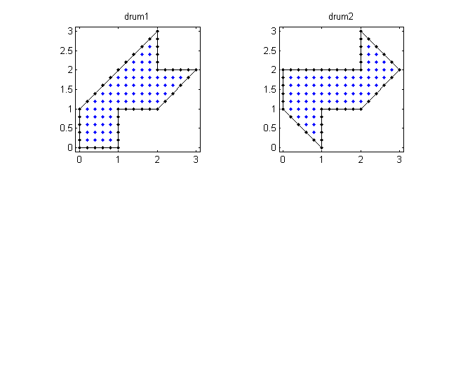
I will look at the simplest known isospectral pair. The two regions are specified by the xy-coordinates of their vertices. drum1 = [0 0 2 2 3 2 1 1 0
0 1 3 2 2 1 1 0 0];
drum2 = [1 0 0 2 2 3 2 1 1
0 1 2 2 3 2 1 1 0];
vertices = {drum1,drum2};
Let's first plot the regions.
   clf
   shg
   set(gcf,'color','white')
   for d = 1:2
      % Plot the region.
      vs = vertices{d};
      subplot(2,2,d)
      plot(vs(1,:),vs(2,:),'k.-');
      axis([-0.1 3.1 -0.1 3.1])
      axis square
      title(sprintf('drum%d',d));
   end
Finite difference grid
I want to investigate simple finite difference methods for this problem. The MATLAB function inpolygon determines the points of a rectangular grid that are in a specified region.% Generate a coarse finite difference grid. ngrid = 5; h = 1/ngrid; [x,y] = meshgrid(0:h:3); % Loop over the two regions. for d = 1:2 % Determine points inside and on the boundary. vs = vertices{d}; [in,on] = inpolygon(x,y,vs(1,:),vs(2,:)); in = xor(in,on); % Plot the region and the grid. subplot(2,2,d) plot(vs(1,:),vs(2,:),'k-',x(in),y(in),'b.',x(on),y(on),'k.') axis([-0.1 3.1 -0.1 3.1]) axis square title(sprintf('drum%d',d)); grid{d} = double(in); end
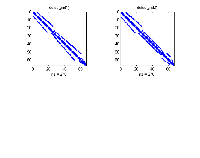
Finite difference Laplacian
Defining the 5-point finite difference Laplacian involves numbering the points in the region. The delsq function generates a sparse matrix representation of the operator and a spy plot of the nonzeros in the matrix shows its the band structure.for d = 1:2 % Number the interior grid points. G = grid{d}; p = find(G); G(p) = (1:length(p))'; % Display the numbering. fprintf('grid%d =',d); minispy(flipud(G)) % Discrete Laplacian. A = delsq(G); % Spy plot subplot(2,2,d) markersize = 6; spy(A,markersize) title(sprintf('delsq(grid%d)',d)); end
grid1 =
  .    .    .    .    .    .    .    .    .    .    .    .    .    .    .    .
  .    .    .    .    .    .    .    .    .    .    .    .    .    .    .    .
  .    .    .    .    .    .    .    .    .   56    .    .    .    .    .    .
  .    .    .    .    .    .    .    .   48   55    .    .    .    .    .    .
  .    .    .    .    .    .    .   41   47   54    .    .    .    .    .    .
  .    .    .    .    .    .   35   40   46   53    .    .    .    .    .    .
  .    .    .    .    .   30   34   39   45   52   60   63   65   66    .    .
  .    .    .    .   26   29   33   38   44   51   59   62   64    .    .    .
  .    .    .   18   25   28   32   37   43   50   58   61    .    .    .    .
  .    .   11   17   24   27   31   36   42   49   57    .    .    .    .    .
  .    5   10   16   23    .    .    .    .    .    .    .    .    .    .    .
  .    4    9   15   22    .    .    .    .    .    .    .    .    .    .    .
  .    3    8   14   21    .    .    .    .    .    .    .    .    .    .    .
  .    2    7   13   20    .    .    .    .    .    .    .    .    .    .    .
  .    1    6   12   19    .    .    .    .    .    .    .    .    .    .    .
  .    .    .    .    .    .    .    .    .    .    .    .    .    .    .    .

grid2 =
  .    .    .    .    .    .    .    .    .    .    .    .    .    .    .    .
  .    .    .    .    .    .    .    .    .    .    .    .    .    .    .    .
  .    .    .    .    .    .    .    .    .    .    .   57    .    .    .    .
  .    .    .    .    .    .    .    .    .    .    .   56   62    .    .    .
  .    .    .    .    .    .    .    .    .    .    .   55   61   65    .    .
  .    .    .    .    .    .    .    .    .    .    .   54   60   64   66    .
  .    5   11   18   26   30   34   38   42   46   50   53   59   63    .    .
  .    4   10   17   25   29   33   37   41   45   49   52   58    .    .    .
  .    3    9   16   24   28   32   36   40   44   48   51    .    .    .    .
  .    2    8   15   23   27   31   35   39   43   47    .    .    .    .    .
  .    1    7   14   22    .    .    .    .    .    .    .    .    .    .    .
  .    .    6   13   21    .    .    .    .    .    .    .    .    .    .    .
  .    .    .   12   20    .    .    .    .    .    .    .    .    .    .    .
  .    .    .    .   19    .    .    .    .    .    .    .    .    .    .    .
  .    .    .    .    .    .    .    .    .    .    .    .    .    .    .    .
  .    .    .    .    .    .    .    .    .    .    .    .    .    .    .    .
Compare eigenvalues
The Arnoldi method implemented in the eigs function readily computes the eigenvalues and eigenvectors. Here are the first twenty eigenvalues.% How many eigenvalues? eignos = 20; % A finer grid. ngrid = 32; h = 1/ngrid; [x,y] = meshgrid(0:h:3); inpoints = (7*ngrid-2)*(ngrid-1)/2; lambda = zeros(eignos,2); V = zeros(inpoints,eignos,2); for d = 1:2 vs = vertices{d}; [in,on] = inpolygon(x,y,vs(1,:),vs(2,:)); in = xor(in,on); % Number the interior grid points. G = double(in); p = find(G); G(p) = (1:length(p))'; grid{d} = G; % The discrete Laplacian A = delsq(G)/h^2; % Sparse matrix eigenvalues and vectors. [V(:,:,d),E] = eigs(A,eignos,0); lambda(:,d) = diag(E); end format long lambda = flipud(lambda)
lambda =

  10.165879621248989  10.165879621248980
  14.630600866993412  14.630600866993376
  20.717633982094981  20.717633982094902
  26.115126153750705  26.115126153750676
  28.983478457829740  28.983478457829762
  36.774063407607322  36.774063407607287
  42.283017757114585  42.283017757114699
  46.034233949715308  46.034233949715386
  49.213425509524733  49.213425509524775
  52.126973962396342  52.126973962396370
  57.063486161172904  57.063486161172769
  63.350675017756465  63.350675017756259
  67.491111510445251  67.491111510445194
  70.371453210957910  70.371453210957810
  75.709992784621988  75.709992784621818
  83.153242199788906  83.153242199788821
  84.673734481953971  84.673734481953886
  88.554340162610174  88.554340162610174
  94.230337192953158  94.230337192953257
  97.356922250794767  97.356922250794653
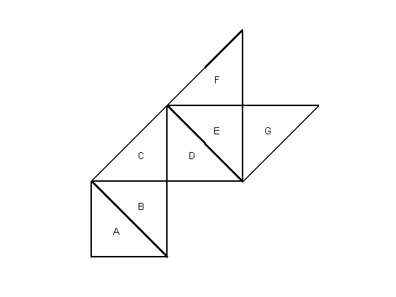
How about a proof?
Varying the number of eigenvalues, eignos, and the grid size, ngrid, in this script provides convincing evidence that the finite difference Laplacians on the two domains are isospectral. But this is not a proof. For the continuous problem, Chapman [8] outlines an approach where any eigenfunction on one of the domains can be constructed from triangular pieces of the corresponding eigenfunction on the other domain. It is necessary to prove that these pieces fit together smoothly and that the differential equation continues to be satisfied across the boundaries. For this proof Chapman refers to a paper by Berard [9]. I will explore the discrete analog of these arguments in a later post.References
- Marc Kac, Can one hear the shape of a drum?, Amer. Math. Monthly 73 (1966), 1-23.
- Cleve Moler, The MathWorks logo is an eigenfunction of the wave equation (2003).
- Lloyd N. Trefethen and Timo Betcke, Computed eigenmodes of planar regions (2005).
- Carolyn Gordon, David Webb, Scott Wolpert, One cannot hear the shape of a drum, Bull. Amer. Math. Soc. 27 (1992), 134-138.
- Wikipedia, Hearing the shape of a drum.
- Tobin Driscoll, Isospectral Drums.
- Tobin Driscoll, Eigenmodes of isospectral drums, SIAM Review 39 (1997), 1-17.
- S. J. Chapman, Drums that sound the same, Amer. Math. Monthly 102 (1995), 124-138.
- Pierre Berard, Transplantation et isospectralite, Math. Ann. 292 (1992), 547-559.
- Category:
- Eigenvalues


Comments
To leave a comment, please click here to sign in to your MathWorks Account or create a new one.