
The Lambert W Function
The Lambert W function deserves to be better known. It pops up in all sorts of places. And our MATLAB function for evaluating the function is a beautiful use of the Halley method.
Contents
Johann Lambert

Johann Henrich Lambert was born in 1728 in Mulhouse, which was then in Switzerland, but is now in France. He was a contemporary of the famous Swiss mathematician Leonard Euler. He had incredibly wide ranging interests. He was the first to prove that $\pi$ was irrational. He introduced the hyperbolic trig functions. He made such important contributions to optics that a photometric unit for luminance is named in his honor. He also made contributions in physics, astronomy, logic, and philosophy.
Lambert did not explicitly describe the function that is now named after him. He considered various equations, including ones of the form $x = q + x^m$. Euler followed up with papers about Lambert's work. The ideas involved in analyzing such equations underlie what we today call the Lambert W function.
The Maple Connection
In the early 1990s developers of the Maple symbolic algebra software, including Rob Corless, Gaston Gonnet, D.E.G. Hare, and David Jeffrey, came to realize that this function had been rediscovered many times over the years. They christened the function "W", published a note in the Maple Technical Newsletter, and began to develop a bibliography. Don Knuth joined the group by contributing applications involving enumerations of trees. In 1996 the five of them wrote a 32 page paper that has become the definitive reference on the Lambert W function. Their bibliography contains 72 entries.
An elementary function
Let's plot an elementary function, using $w$ as the independent variable. The function is $w \mbox{e}^w$.
   f = @(w) w.*exp(w);
   ezplot(f,[-4 1])
   xlabel('w')
   axis([-4 1 -.5 1])
   axis square
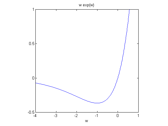
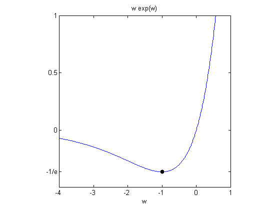
You can see the function reaches a global minimum at $w = -1$. The value of this minimum plays an important role in this story, so let's give it a name.
$$ \bar{\mbox{e}} = -1/\mbox{e} $$
   ebar = -1/exp(1)
   line([-1,-1],[ebar,ebar],'marker','.','markersize',18,'color','black')
   set(gca,'ytick',[ebar,0,0.5,1])
   set(gca,'yticklabel',{'-1/e','0','0.5','1'})
ebar =
  -0.367879441171442
Functional inverse
The Lambert W function, $W(x)$, is the functional inverse of $w \mbox{e}^w$. In other words, $w$ = W($x$) is the solution of the equation
$$ x = w \mbox{e}^w $$
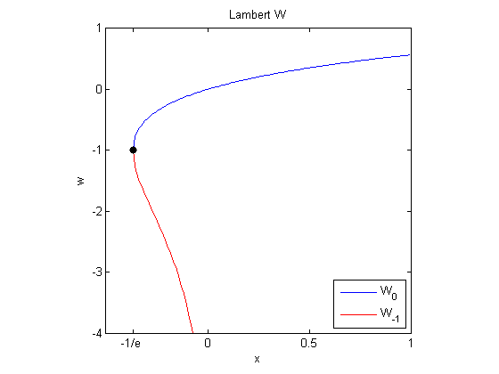
The graph of $W(x)$ is conceptually obtained by labeling the vertical axis of the above graph with an 'x' and then interchanging the horizontal and vertical axes. (You can sneak a peak at the actual plot below, generated after we see how to compute the function.)
The point $x = \bar{\mbox{e}} = -1/\mbox{e}$ is crucial. On the interval $\bar{\mbox{e}} <= x <= 0$ there are two real solutions and so $W(x)$ is double valued. One solution is increasing, is defined for all $x >= \bar{\mbox{e}}$, is known is the primary branch, and is denoted by $W_0(x)$. The other solution is decreasing, is defined only for negative $x$, has a pole at 0, and is denoted by $W_{-1}(x)$. (There are other, complex-valued, branches, $W_k(x)$, which we are not considering here.)
Halley's method
Halley's method is a method for finding a zero of a real-valued function with a continuous and easily computed second derivative. It is named after the British astronomer who is better known for discovering a comet.
Newton's method approximates a function locally by a linear function with the same slope and steps to the zero of that approximation. Halley's method approximates the function locally by a hyperbola with the same slope and curvature and steps to the nearest zero of that approximation. The iteration is
$$w_{n+1}=w_n-f(w_n)/\left[f'(w_n)-\frac{f(w_n)f''(w_n)}{2f'(w_n)}\right]$$
You can see Newton's method by ignoring the second term in the square brackets. You can see that Halley's method is particularly efficient if the ratio $f''(w)/f'(w)$ happens to take a simple form. But we do not regard Halley's method as a general purpose method because it does require knowledge of the second derivative.
Application to Lambert W
Computing $W(x)$ for a given value of $x$ requires solving the equation
$$ f(w) = w \mbox{e}^w - x = 0 $$
for $w$. We can use Halley's method because the required derivatives are readily available.
$$ f'(w) = w \mbox{e}^w + \mbox{e}^w = \mbox{e}^w (w + 1) $$
$$ f''(w) = w \mbox{e}^w + w \mbox{e}^w + \mbox{e}^w = \mbox{e}^w (w + 2) $$
Note that
$$ f''(w)/f'(w) = (w+2)/(w+1) $$
This gives us the following iterative step for computing Lambert W at a given value of $x$.
$$ f_n = w_n \mbox{e}^{w_n} - x $$
$$w_{n+1}=w_n-f_n/\left[\mbox{e}^{w_n}(w_n+1)-(w_n+2)f_n/(2 w_n+2)\right]$$
Starting values
Various people have written programs before me to compute Lambert W using Halley's method. They have paid quite a bit of attention to starting values that reduce the eventual number of iterations. I have decided to take a different approach. I am willing to have the computation take a few more iterations if the program can be simplified. In fact, I use the simplest possible initial values.
For the primary branch, start with $w = 1$ for any $x$. Do not try to approximate $W(x)$ at all. The iteration turns out to converge to double precision floating point accuracy in about a half dozen iterations for any $x$, except values very near the branch point at $\bar{\mbox{e}}$. More accurate starting values could cut the number of iterations in half, but I prefer the simpler code.
For the lower branch, start with any value less than $-1$. I have chosen $w = -2$, but I don't think it matters very much. Again, about a half dozen iterations are required unless $x$ is very close to the branch point at $\bar{\mbox{e}}$ or the pole at $0$.
Stopping values
Halley's method is cubically convergent near a simple root, which this is. Once we're close, we get closer very fast. If two successive iterates agree to 1.0e-8, then you can be pretty sure the second one is accurate to 1.0e-16. I could probably even replace 1.e-8 by eps^(1/3) = 6e-6.
Lambert_W.m
Here is the entire M-file for function Lambert_W. This will be available from the MATLAB Central File Exchange in due course. (Added 9/16/2013: See this link)
type Lambert_W
function w = Lambert_W(x,branch)
% Lambert_W  Functional inverse of x = w*exp(w).
% w = Lambert_W(x), same as Lambert_W(x,0)
% w = Lambert_W(x,0)  Primary or upper branch, W_0(x)
% w = Lambert_W(x,-1)  Lower branch, W_{-1}(x)
%
% See: https://blogs.mathworks.com/cleve/2013/09/02/the-lambert-w-function/

% Copyright 2013 The MathWorks, Inc.

% Effective starting guess
if nargin < 2 || branch ~= -1
   w = ones(size(x));  % Start above -1
else
   w = -2*ones(size(x));  % Start below -1
end
v = inf*w;

% Haley's method
while any(abs(w - v)./abs(w) > 1.e-8)
   v = w;
   e = exp(w);
   f = w.*e - x;  % Iterate to make this quantity zero
   w = w - f./((e.*(w+1) - (w+2).*f./(2*w+2)));
end
Plot Lambert W
We can now use this code to produce a plot of both branches of the Lambert W function.
% Primary branch

   x = ebar:.01:1;
   plot(x,Lambert_W(x,0))

% Lower branch

   hold on
   x = ebar:.01:0;
   plot(x,Lambert_W(x,-1),'r')
   hold off

% Annotation

   axis([-.5 1 -4 1])
   axis square
   line([ebar ebar],[-1 -1],'marker','.','markersize',18,'color','black')
   set(gca,'xtick',[ebar 0 .5 1])
   set(gca,'xticklabel',{'-1/e','0','0.5','1'})
   set(gca,'ytick',-4:1)
   xlabel('x')
   ylabel('w')
   title('Lambert W')
   legend({'W_0','W_{-1}'},'location','southeast')
Acknowledgements
Thanks to Peter Costa for reawakening my interest and to Rob Corless for keeping me up to date as always.
Lambert W Poster
Follow this link to a poster about the Lambert W function produced by the group at the University of Western Ontario led by Corless and Jeffrey.
Further Reading
Corless, R., Gonnet, G., Hare, D., Jeffrey, D., Knuth, Donald (1996). "On the Lambert W function". Advances in Computational Mathematics (Berlin, New York: Springer-Verlag) 5: 329-359. <http://link.springer.com/article/10.1007%2FBF02124750>
Corless, R., Gonnet, G., Hare, D., Jeffrey, D., Knuth, Donald (1996). "On the Lambert W function". PDF Preprint. https://cs.uwaterloo.ca/research/tr/1993/03/W.pdf
Wikipedia article. <http://en.wikipedia.org/wiki/Lambert_W_function>
NIST Digital Library of Mathematical Functions. <http://dlmf.nist.gov/4.13>
Halley's Method: Dahlquist, G., Bjorck, A. Numerical Methods in Scientific Computing, Volume I, page 648, SIAM, Philadelphia, 2008.


Comments
To leave a comment, please click here to sign in to your MathWorks Account or create a new one.