
Benchmarking a GPU
I recently acquired a GPU, a graphics processing unit. It's called a GPU because such processors were originally intended to speed up graphics. But MATLAB uses it to speed up computation. Let's see how the gpuArray object benchmarks on my machine.
I have been doing computer benchmarks for years. I like to do profiles where I vary the size of a task and see how the amount of memory required affects performance. I always learn something unexpected when I do these profiles.
Ben Todoroff is on the MathWorks Parallel Processing team. Last year he contributed #34080, gpuBench to the MATLAB Central File Exchange. He has been able to compare several different GPUs. I am going to consider the performance of only one GPU, but in more detail.
Important note. This is only about double precision. Single precision is another story.
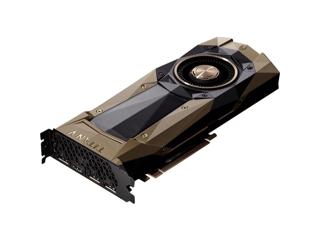 Image credit: NVIDIA
 The operating frequency varies automatically between the rated base speed of 1.90 GHz and well over 3 GHz. This gets throttled up and down in response to temperature changes and who knows what else. The machine runs faster when I first power it up on a cold morning than it does later in the day.
Notice the 8 percent utilization by 239 processes and 3026 threads. I know that most of these threads are idle, waiting to wake up and interfere with my timing experiments. All I can do is run things many times and take an average. Or maybe I should use the minimum time, like a sprinter's personal best.
The operating frequency varies automatically between the rated base speed of 1.90 GHz and well over 3 GHz. This gets throttled up and down in response to temperature changes and who knows what else. The machine runs faster when I first power it up on a cold morning than it does later in the day.
Notice the 8 percent utilization by 239 processes and 3026 threads. I know that most of these threads are idle, waiting to wake up and interfere with my timing experiments. All I can do is run things many times and take an average. Or maybe I should use the minimum time, like a sprinter's personal best.
 The times are increasing like n^3, as expected. For A\b the inner loop is executed roughly 2/3 n^3 times, so gigaflops are
 I conclude that for x = A\b my machine reaches about 70 gigaflops for n = 10000 and doesn't speed up much for larger matrices.
 So matrix multiply on the CPU can reach over 80 gigaflops for order as small as 2000.
 There is a discontinuity, probably a cache size effect, around n = 8000.
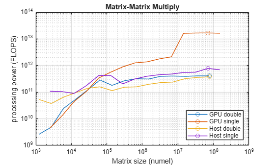
 A pair of matrices as large as order 14000 can be multiplied in less than a second. Six teraflops is the top speed. We reach that by order 3000.
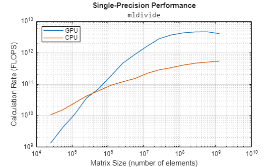
 The CPU is faster than the GPU for linear systems of order 789 or smaller. The GPU can up to 15 times faster than the CPU, until it runs out of memory. Of course, this is not counting any data transfer time.
 As a function of matrix order, both the CPU and the GPU reach their top speeds quickly. Then it is 80 gigaflops versus 6 teraflops. The GPU is 75 times faster.
Contents
My Laptop
The laptop where I do most of my work is a ThinkPad T480s, with an Intel Core i7-8650U processor having a base operating frequency of 1.90 GHz. The CPU has four cores and a maximum Turbo frequency of 4.20 GHz. There is 16GB of main memory. I run the Microsoft Windows 10, 64-bit operating system. The retail price is around $1500. MATLAB uses the Intel Math Kernel Library, which is multithreaded. So, it can take advantage of all four cores.GPU
The GPU is an NVIDIA Titan V operating at 1.455 GHz. It has 12GB of memory, 640 Tensor cores and 5120 CUDA cores. It is housed in a separate Thunderbolt peripheral box which is several times larger than the laptop itself. This box has its own 240W power supply and a couple of fans. It retails for $2999.
Image credit: NVIDIA
Benchmarking
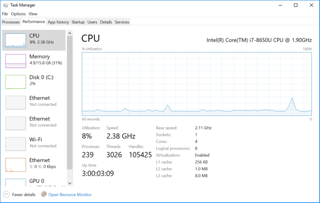
This has been a frustrating project. Trying to measure the speed of modern computers is very difficult. I can bring up the Task Manager performance meter on my machine. I can switch on airplane mode so that I am no longer connected to the Internet. I can shut down MATLAB and close all other windows, except the perf meter itself. I can wait until all transient activity is gone. But I still don't get consistent times. Here is a snapshot of the Task Manager.
The operating frequency varies automatically between the rated base speed of 1.90 GHz and well over 3 GHz. This gets throttled up and down in response to temperature changes and who knows what else. The machine runs faster when I first power it up on a cold morning than it does later in the day.
Notice the 8 percent utilization by 239 processes and 3026 threads. I know that most of these threads are idle, waiting to wake up and interfere with my timing experiments. All I can do is run things many times and take an average. Or maybe I should use the minimum time, like a sprinter's personal best.
Flops
I'm going to be measuring gigaflops. That's 10^9 flops. What is a flop? The inner loops of most matrix computations are either dot products,s = s + x(i)*y(i)or "daxpys", double a x plus y,
y(i) = a*x(i) + y(i)In either case, that's one multiplication, one addition, and a handful of indexing, load and store operations. Taken altogether, that's two floating point operations, or two flops. Each time through an inner loop counts as two flops. If we ignore cache and memory effects, the time required for a matrix computation is roughly proportional to the number of flops.
CPU, A\b
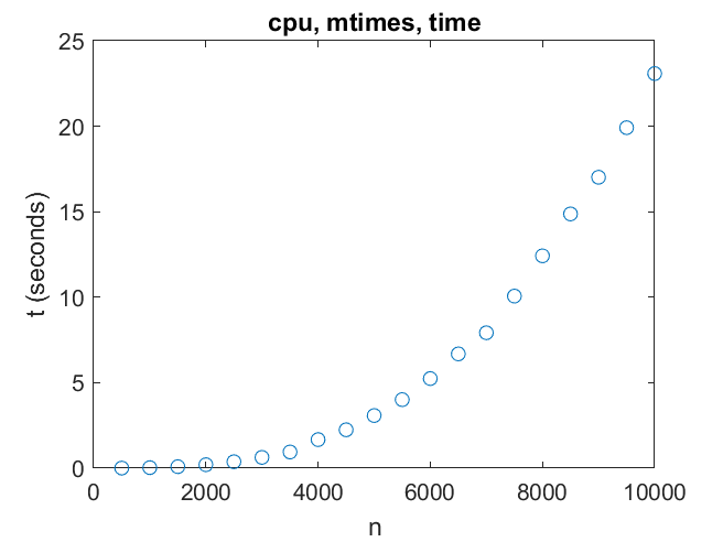
Here is a typical benchmark run for timing the iconic x = A\b.t = zeros(1,30); m = zeros(1,30); n = 0:500:15000; tspan = 1.0;
while ~get(stop,'value')
   k = randi(30);
   nk = n(k);
   A = randn(nk,nk);
   b = randn(nk,1);
   cnt = 0;
   tok = 0;
   tic
   while tok < tspan
       x = A\b;
       cnt = cnt + 1;
       tok = toc;
   end
   t(k) = t(k) + tok/cnt;
   m(k) = m(k) + 1;
end
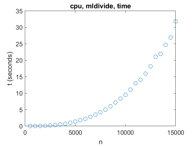
t = t./m;
gigaflops = 2/3*n.^3./t/1.e9;
This randomly varies the size of the matrix between 500-by-500 and 15,000-by-15,000. If it takes less than one second to compute A\b, the computation is repeated. It turns out that systems of order 3000 and less need to be repeated. At the two extremes, systems of order 500 need to be repeated over 100 times, while systems of order 15,000 require over 30 seconds. If I run this for more than an hour, each value of n is encountered several times and the average times settle down. After adding some annotation to
plot(n,t,'o')I get
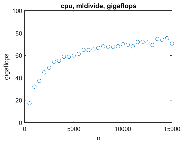
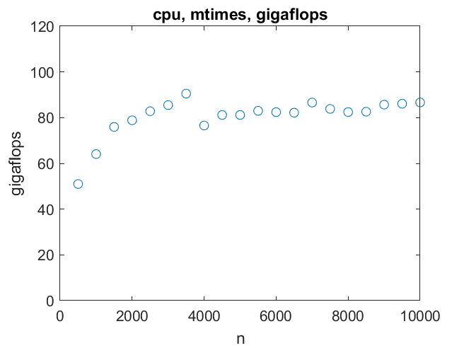
The times are increasing like n^3, as expected. For A\b the inner loop is executed roughly 2/3 n^3 times, so gigaflops are
giga = 2/3*n.^3./t/1.e9
I conclude that for x = A\b my machine reaches about 70 gigaflops for n = 10000 and doesn't speed up much for larger matrices.
CPU, A*B
Multiplication of two n -by- n matrices requires 2n^3 flops, three times as many as solving one linear system.
So matrix multiply on the CPU can reach over 80 gigaflops for order as small as 2000.
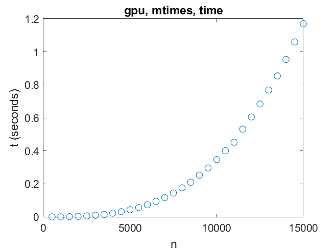
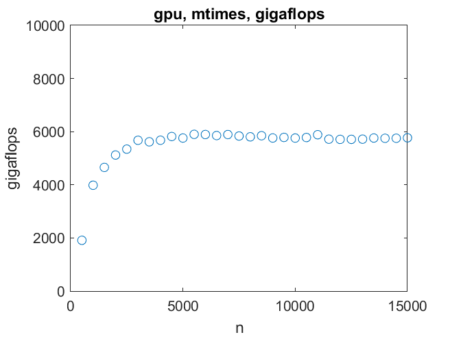
GPU, A\b
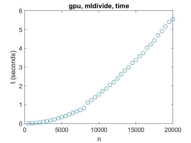
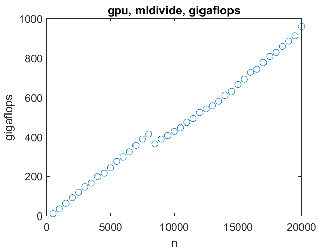
Now to the primary motivation for this project, the GPU. First, solving a linear system. Here we reach a significant obstacle -- there is only enough memory on this GPU to handle linear systems of order 21000 or so. For such systems the performance can reach one teraflop (10^12 flops). That is nowhere near the speed that could be reached if there were more memory for the GPU.
There is a discontinuity, probably a cache size effect, around n = 8000.
GPU, A*B
It is easy to break matrix multiplication into many small, parallel tasks that the GPU can handle.
A pair of matrices as large as order 14000 can be multiplied in less than a second. Six teraflops is the top speed. We reach that by order 3000.
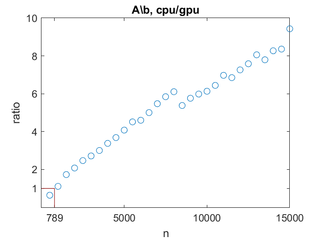
A\b, Comparison
How does the GPU compare to the CPU on A\b?
The CPU is faster than the GPU for linear systems of order 789 or smaller. The GPU can up to 15 times faster than the CPU, until it runs out of memory. Of course, this is not counting any data transfer time.
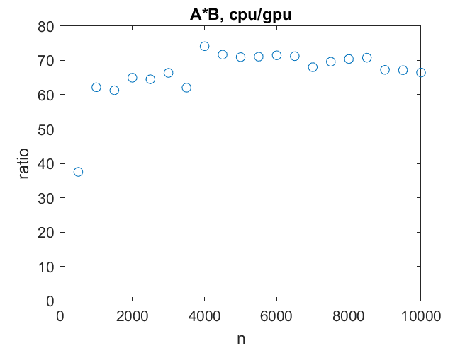
A*B, Comparison
The story is very different for matrix multiplication.
As a function of matrix order, both the CPU and the GPU reach their top speeds quickly. Then it is 80 gigaflops versus 6 teraflops. The GPU is 75 times faster.
Supercomputers, Then and Now
Over 40 years ago, at the beginnings of the LINPACK Benchmark, the fastest supercomputer in the world was the newly installed Cray-1 at NCAR, the National Center for Atmospheric Research in Boulder. That machine could solve a 100-by-100 linear system in 50 milliseconds. That's 14 megaflops (10^6 flops), about one-tenth of its top speed of 160 megaflops. At 6 teraflops, the machine on my desk is 37,500 times faster. Both the Cray-1 and the NVIDIA Titan V could profit from more memory. On the other hand, the fastest supercomputer in the world today is Summit, at Oak Ridge National Laboratory in Tennessee. Its 200 petaflops (10^15 flops) top speed in roughly 37,500 times faster than my laptop plus GPU. And, Summit has lots of memory.Published with MATLAB® R2018b


Comments
To leave a comment, please click here to sign in to your MathWorks Account or create a new one.