
Roundoff Patterns from Triple Kronecker Products
While I was working on my posts about Pejorative Manifolds, I was pleased to discover the intriguing patterns created by the roundoff error in the computed eigenvalues of triple Kronecker products.
Contents
Kronecker Product
The Kronecker product of two matrices $A$ and $B$, denoted by $A \otimes B$ and computed by kron(A,B), is the large matrix containing all possible products of the elements of $B$ by those of $A$.
$$A \otimes B = \left( \begin{array}{rrrr} a_{1,1}B & a_{1,2}B & ... & a_{1,n}B \\ a_{2,1}B & a_{2,2}B & ... & a_{2,n}B \\ ... \\ a_{m,1}B & a_{m,2}B & ... & a_{m,n}B \end{array} \right) $$
The two matrices $A \otimes B$ and $B \otimes A$ are not equal, although they do have the same elements in different orders.
The two matrices $A \otimes (B \otimes C)$ and $(A \otimes B) \otimes C$ are equal. This is the triple Kronecker product, $A \otimes B \otimes C$.
The eigenvalues of $A \otimes B$ are all possible products of the eigenvalues of $A$ and those of $B$.
Example
For example, suppose $A$ is the magic square.
$$ A = \left( \begin{array}{rrr} 8 & 1 & 6 \\ 3 & 5 & 7 \\ 4 & 9 & 2 \end{array} \right) $$
And $I$ is the identity matrix.
$$ I = \left( \begin{array}{rr} 1 & 0 \\ 0 & 1 \end{array} \right) $$
Then $I \otimes A$ is block diagonal with copies of $A$ on the diagonal.
$$ I \otimes A = \left( \begin{array}{rrrrrr} 8 & 1 & 6 & 0 & 0 & 0 \\ 3 & 5 & 7 & 0 & 0 & 0 \\ 4 & 9 & 2 & 0 & 0 & 0 \\ 0 & 0 & 0 & 8 & 1 & 6 \\ 0 & 0 & 0 & 3 & 5 & 7 \\ 0 & 0 & 0 & 4 & 9 & 2 \end{array} \right) $$
And $A \otimes I$ has the elements of $A$ distributed along multiple diagonals.
$$ A \otimes I = \left( \begin{array}{rrrrrr} 8 & 0 & 1 & 0 & 6 & 0 \\ 0 & 8 & 0 & 1 & 0 & 6 \\ 3 & 0 & 5 & 0 & 7 & 0 \\ 0 & 3 & 0 & 5 & 0 & 7 \\ 4 & 0 & 9 & 0 & 2 & 0 \\ 0 & 4 & 0 & 9 & 0 & 2 \end{array} \right) $$
The eigenvalues of both $A\otimes I$ and $I \otimes A$ are multiple copies of the eigenvalues of $A$.
   A = magic(3);
   I = eye(2);
   eig_A = eig(A)
   eig_IxA = eig(kron(I,A))
   eig_AxI = eig(kron(A,I))
eig_A =
  15.000000000000004
   4.898979485566361
  -4.898979485566358
eig_IxA =
  15.000000000000004
   4.898979485566361
  -4.898979485566358
  15.000000000000004
   4.898979485566361
  -4.898979485566358
eig_AxI =
   4.898979485566356
  -4.898979485566355
  15.000000000000002
  14.999999999999998
   4.898979485566359
  -4.898979485566356
Eigenvalues with high multiplicity
Our building blocks are the companion matrices of the polynomials
$$ (s^2-1)^p $$
Expansion involves binomial coefficients. For example, p = 4,
$$ (s^2-1)^4 = s^8 - 4 s^6 + 6 s^4 - 4 s^2 + 1 $$
This is the characteristic polynomial of the matrix
A = companion(4)
A =
     0     4     0    -6     0     4     0    -1
     1     0     0     0     0     0     0     0
     0     1     0     0     0     0     0     0
     0     0     1     0     0     0     0     0
     0     0     0     1     0     0     0     0
     0     0     0     0     1     0     0     0
     0     0     0     0     0     1     0     0
     0     0     0     0     0     0     1     0
The eigenvalues of A are +1 and -1, each repeated p times; that's their algebraic multiplicity. Their geometric multiplicity is only one; they have only one eigenvector each.
The eigenvalues are very sensitive to any kind of error, including roundoff error.
   format long
   e = eig(A)
e =
 -1.000063312800363 + 0.000063312361825i
 -1.000063312800363 - 0.000063312361825i
 -0.999936687199636 + 0.000063313248591i
 -0.999936687199636 - 0.000063313248591i
  1.000078270656946 + 0.000000000000000i
  0.999999997960933 + 0.000078268622898i
  0.999999997960933 - 0.000078268622898i
  0.999921733421185 + 0.000000000000000i
The exact eigenvalues can be recovered with
exact = round(e)
exact =
    -1
    -1
    -1
    -1
     1
     1
     1
     1
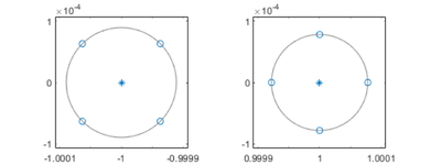
The computed eigenvalues lie on circles in the complex plane, centered at the exact values, with radius roughly the p-th root of roundoff error. In this example, the values centered at +1 happen to be slightly more accurate than those centered at -1.
   half_fig
   eigplot(-1,e)
   eigplot(+1,e)
Fiedler companion matrix
An alternative to the traditional companion matrix is the Fiedler companion matrix.
A = companion(4,'fiedler')
A =
     0     4     1     0     0     0     0     0
     1     0     0     0     0     0     0     0
     0     0     0    -6     1     0     0     0
     0     1     0     0     0     0     0     0
     0     0     0     0     0     4     1     0
     0     0     0     1     0     0     0     0
     0     0     0     0     0     0     0    -1
     0     0     0     0     0     1     0     0
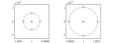
This time the eigenvalues are computed in the opposite order and those at -1 are the more accurate.
e = eig(A)
e =
  1.000107000301506 + 0.000000000000000i
  1.000000000805051 + 0.000107001107366i
  1.000000000805051 - 0.000107001107366i
  0.999892998088390 + 0.000000000000000i
 -1.000062156379228 + 0.000000000000000i
 -0.999999990704846 + 0.000062147083463i
 -0.999999990704846 - 0.000062147083463i
 -0.999937862211083 + 0.000000000000000i
   e = flipud(e);
   half_fig
   eigplot(-1,e)
   eigplot(+1,e)
Triple Kronecker Product
Our graphic TKP involves $K$, the triple Kronecker matrix product
$$ K = A \otimes I \otimes B $$
where $A$ and $B$ are companion matrices of the polynomials $(s^2-1)^p$ and $(s^2-1)^r$ and $I$ is the $q$ -by- $q$ identity matrix.
The values of p, q and r are set by controls. Initially they are equal to 4, 3 and 2. The size of $K$ is four times the product of the three sizes, n = 4pqr. Computation time is $O(n^3)$. Values of n larger than about 4000 are possible, but slow.
Half of the eigenvalues of $K$ are equal to +1 and the other half are equal to -1, so these eigenvalues have very high multiplicity and are very sensitive to roundoff error. The display shows the differences between the computed and the exact eigenvalues. The structure of $K$ makes these errors produce provocative patterns on many different circles in the complex plane.
Two kinds of companion matrix with different roundoff behavior are possible. The traditional companion matrix has all the polynomial coefficients in the first row of an upper Hessenberg matrix. The Fiedler companion matrix has the coefficients arranged on the super and subdiagonals of a pentadiagonal matrix.
TKP
This is the computational core. The complete program with the controls is available here: tkp.m.
function tkp(p,q,r)
    A = companion(p);
    I = eye(q);
    B = companion(r);
    K = kron(A,kron(I,B));
    e = eig(K);
    exact = round(e);
    err = e - exact;
    plot(err,'.')
end
function X = companion(p)
    c = 1;
    for j = 1:p
        c = conv(c,[1 0 -1]);
    end
    m = 2*p;
    X = [-c(2:m+1); eye(m-1,m)];
end
- Category:
- Eigenvalues,
- Fun,
- Graphics,
- Matrices,
- Numerical Analysis


Comments
To leave a comment, please click here to sign in to your MathWorks Account or create a new one.