Alexa tells me that the definition of serendipity is "the occurrence and development of events by chance in a happy or beneficial way."

Contents

Smale Birthday

As I have mentioned before in this blog, Indika Rajapakse from Ann Arbor, Stephen Smale from Berkeley and I are working on a project about the Kuramoto model of self-synchronizing oscillators. Steve's birthday was last week and Indika organized a Zoom conference call involving over 100 of Steve's friends to wish him "Happy Birthday." During the celebration, I initiated a private Zoom chat with another Steve, Steven Strogatz from Cornell, who is an expert on Kuramoto. Strogatz and I decided to have a one-on-one Zoom video call the next day.

Locking Threshold

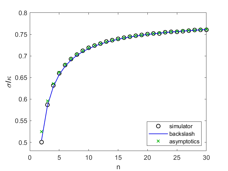
My Kuramoto simulator uses ode45 to solve Kuramoto's equations and investigate the behavior of the dynamical system. Several months ago, I computed the values of something called the locking threshold for a system of $n$ oscillators. These values are the circles in this plot. Let's denote them by $s_n$.

Strogatz asymptotic analysis

In our Zoom call, Strogatz told me about his 2016 paper with Bertrand Ottino-Loffler, Kuramoto model with uniformly spaced frequencies. In this paper, they prove the following impressive result about the asymptotic behavior of the locking threshold a function of $n$.

$$\gamma_L = \frac{\pi}{4} - \frac{\pi}{4} n^{-1} + 4 \zeta(-\frac{1}{2},\frac{C_1}{2}) n^{-3/2} + O(n^{-2}) $$

where $\zeta(s,q)$ is the Hurwitz generalization of the Riemann zeta function and $C_1$ is the QRS constant analyzed by David Bailey, Jon Borwein and Richard Crandall in a paper in Experimental Mathematics.

Well, I was blown away. Where did that $\pi$ come from? How did the power $n^{-3/2}$ get there? What are the Hurwitz zeta function and the QRS constant? I couldn't answer any of these questions.

Data fit

Undaunted, I tried fitting my computed values $s_n$ with a function of the form

$$ s_n \approx \frac{\pi}{4} - \frac{\pi}{4} n^{-1} + c n^{-3/2} $$

I found c = 0.3185 and the resulting blue line in the plot. It is a beautiful fit. I was excited.

Serendipity

Now the serendipity part. It turns out that I've known Dave Bailey for a long time. He has made numerous contributions to high performance computing, including the venerable NAS Benchmark. I was at the 1993 meeting when he and the Borwein brothers, Jon and Peter, received the Chauvenet Prize for expository writing honoring their paper about how to compute a billion digits of $\pi$. At that meeting, the Borwein's told me about the six consecutive 9s around location 780 in the decimal expansion of $\pi$.

I also knew Richard Crandall. He was a professor at Reed College in Portland, Oregon. He had a long association with Steve Jobs, dating back to Jobs' stint as a student at Reed in the '70s. Crandall actually had a summer job working for me when I was at the Intel Hypercube operation in Beaverton, Oregon in the '80s.

Asymptotics

Getting back to Kuramoto, after I had done my curve fit, I read the Strogatz paper more thoroughly. It is a skillful and detailed analysis involving sums converging to integrals. On the last page I found the approximate numerical value, 0.3735, for the coefficient of the $n^{-3/2}$ term in the asymptotic series. That leads to the green x's in my plot, which are amazingly close to the values in the circles since the series is intended to apply as $n \rightarrow \infty$ and I am evaluating it starting with $n = 2$.

Backslash

How did I compute the coefficient c = .3125? Let s be the 29-by-1 MATLAB column vector of computed locking thresholds.

   s = kuramoto_locking_thresholds;

Let n be the column vector of corresponding number of oscillators.

   n = (2:30)';

Then

   t = pi/4*(1 - 1./n);

is the first two terms in the asymptotic series. Also let

   p = n.^(-3/2);

I want to find the scalar c so that t + c*p is as close as to s as possible. This an overdetermined system of 29 linear equations with only one unknown.

$$\texttt{p*c} \approx \texttt{s-t}$$

How do you "solve" such an equation with MATLAB? The least squares solution is computed by backslash.

   c = p\(s-t)

c =

    0.3185

This gives me the blue line in the graphic.

   fit = t + c*p;

Get the MATLAB code

Published with MATLAB® R2020b