Analyzing Baby Names with MATLAB R2015b
Today's guest blogger is Matt Tearle, from the Training Services group here at MathWorks. Matt puts two data analysis functions introduced in R2015b through their paces with some unexpected uses.
Contents
Introducing two new functions
Our tireless MATLAB developers keep adding great new functionality for data analysis. I've been having fun playing with two new functions introduced in R2015b: findgroups and splitapply. These functions make it easy to find all unique combinations of key variables, assign a group number to each observation in your data based on those key variables, then apply a function to each of those groups.
The documentation and the release video show examples of the standard, expected use, such as finding the median blood pressure measurement of patients in a trial, grouped by the patients' gender and the drug dosage they received. Let's make a table of some simulated data for this drug trial example.
rng(1234)
numpatients = 15;
gender = categorical(randi(2,numpatients,1),1:2,{'F','M'});
drugdose = 50*randi(3,numpatients,1);
bp = 100 + 40*rand(numpatients,1);
patientdata = table(gender,drugdose,bp,'VariableNames',{'Gender','Dose','BP'})
patientdata =
    Gender    Dose      BP
    ______    ____    ______
    F         100     134.77
    M         100     117.45
    F          50     132.09
    M         150     105.75
    M         150     128.17
    F         100     128.18
    F         100     108.75
    M          50     136.99
    M         100     117.69
    M         150     136.37
    F         100     102.39
    M         100     107.37
    M         150     101.89
    M          50        127
    F         100     123.78
First use findgroups to assign a group number to each patient, where the groups are defined by the combination of Gender and Dose. It's then easy to calculate the median of BP for each group using splitapply.
group = findgroups(patientdata(:,{'Gender','Dose'}));
medianbp = splitapply(@median,patientdata.BP,group)
medianbp =
       132.09
       123.78
       131.99
       117.45
       116.96
Note that there are five values, even though there are six possible combinations of gender and drug dose. You can use the second output from findgroups to obtain the list of groups. Because the input is a table, the group names will also be returned as a table. You can use dot notation indexing to add the median blood pressure values to the table.
[group,gender_and_dose] = findgroups(patientdata(:,{'Gender','Dose'}));
gender_and_dose.MedianBP = splitapply(@median,patientdata.BP,group)
gender_and_dose =
    Gender    Dose    MedianBP
    ______    ____    ________
    F          50     132.09
    F         100     123.78
    M          50     131.99
    M         100     117.45
    M         150     116.96
One of best things about my job is that I get to see these new features take shape and think about how MATLAB users (like you!) can put them to work. What's really fun is when I get to use the features myself for my own work. Or play. And what's really really fun is when that usage employs a little "out-of-the-box" thinking. In this case, I think I discovered applications for findgroups and splitapply that were not quite what the developers had in mind.
Popular baby names, from Aagot to Zzyzx
Maybe there's something in the water in our building, but a lot of coworkers are having babies. This naturally leads to many coffee-machine conversations about baby stuff: sleep deprivation, busybody in-laws, and, of course, names.
One particular conversation turned to common and uncommon baby names. (My own kids are in the former category, and a coworker's is in the latter.) Being the data-driven MATLAB nerds that we are, we figured there must be a way to quantify just how common a given name is. I recalled that, for the U.S., the Social Security Administration keeps records of baby names. A minute or two with a well-known internet search engine and I had my data source -- a zip file containing names and numbers for each year from 1880 to 2014. All I had to do was read the data from these files into MATLAB, and I'd be able to find out where any given name ranked in all-time popularity.
Each file in the downloaded folder contained data for a given year and consisted of three columns: name, gender, and the number of children (of that gender) registered with that name in that year. The first few lines of the file for 1880 look like this:
dbtype('names\yob1880.txt','1:8')
1     Mary,F,7065
2     Anna,F,2604
3     Emma,F,2003
4     Elizabeth,F,1939
5     Minnie,F,1746
6     Margaret,F,1578
7     Ida,F,1472
8     Alice,F,1414
And 1980 looks like this:
dbtype('names\yob1980.txt','1:8')
1     Jennifer,F,58385
2     Amanda,F,35820
3     Jessica,F,33920
4     Melissa,F,31631
5     Sarah,F,25741
6     Heather,F,19971
7     Nicole,F,19916
8     Amy,F,19832
Note that the names are not in the same order from year to year (they are in order of popularity for that year). Different files do not even contain the same list of names. In 2010 there were 5 boys called Zzyzx, and in 1915 there were 5 girls called Aagot; in no other years were either of these names popular enough to reach the 5-name cutoff.
Reading any one file into MATLAB is easy -- it's just delimited text. But how should I compile the data from all years into one array? This actually depends on how I plan to use the data. If I want to study patterns through time, I'd need to make a table of names with annual counts, like this:
      |  Mary   Anna  ...  Aagot  ...
------|-------------------------------
 1880 |  7065   2604  ...      0  ...
 1881 |  6919   2698  ...      0  ...
 ...  |               ...
 1915 | 58187  15120  ...      5  ...
 ...  |               ...
There are ways to accomplish this using tables, which are another (somewhat) new feature of MATLAB that I love and frequently use for my own work. But in this case, I didn't need the individual annual values; I just needed the all-time totals. It occurred to me that if I had all the data concatenated into one big list, then I'd just need to combine all the repeated name/gender combinations:
Mary,F,7065      <------|
Anna,F,2604             |
Emma,F,2003             |
...                     |
Mary,F,6919      <------|
Anna,F,2698             |
...                     |--- sum --> Total number of girls called Mary
Mary,F,58187     <------|
Helen,F,30866           |
Dorothy,F,25154         |
...                     |
Liliana,F,2624          |
Mary,F,2611      <------|
Elena,F,2598
...
By now hopefully you're seeing what I saw: findgroups and splitapply can actually be applied to collate my data. The groups will be the combinations of name and gender. The function to apply will be sum and the data to apply it to will be the number.
Putting theory into practice
Now all I need is to get all the data in as one big table. It turns out that this is very easy using another recent MATLAB feature: datastores. Datastores are designed to make it easy to read data from multiple files with the same formatting. In this case, all the files are comma-delimited text with three columns.
dat = datastore('names\yob*.txt',...
    'ReadVariableNames',false,'VariableNames',{'Name','Gender','Number'});
This creates a datastore that refers to all the data files. The options specify the variable names for the three columns, rather than obtain them by reading a header line in the file (these files do not contain any header information). The format for each column has been determined automatically. But rather than read the gender as a string, I can modify the format to read it as a categorical variable:
dat.SelectedFormats{2} = '%C';
Categorical variables are easier and more efficent to work with than strings, when dealing with a large number of instances of a small number of unique strings ('F' and 'M', in this case).
Now I'm ready to read the data. I can read each file individually with the read function, but I can also read everything in one go with the readall function:
rawnamedata = readall(dat);
whos rawnamedata
  Name                   Size                Bytes  Class    Attributes

  rawnamedata      1825433x3             243420481  table
Wow. Importing data has never been so easy! Now that I have all the data in one table, I can use findgroups to find all name/gender combinations and assign groups accordingly:
[group,names] = findgroups(rawnamedata(:,{'Name','Gender'}));
And, finally, splitapply to collate the totals:
names.Number = splitapply(@sum,rawnamedata.Number,group);
whos names
  Name            Size               Bytes  Class    Attributes

  names      104110x3             13943724  table
Now names is a table like rawnamedata but with all the repeats for each name totalled into a single observation.
It's now straightforward to obtain the all-time number for any given name. I can leave the names as strings, which allows for all sorts of string matching ("names starting with 'Aa'"), or convert them to categorical, which allows only exact matching but with == instead of strcmp.
names.Name = categorical(names.Name);
names(names.Name == 'Loren',:)
names(names.Name == 'Cleve',:)
ans =
    Name     Gender    Number
    _____    ______    ______
    Loren    F         11862
    Loren    M         45806
ans =
    Name     Gender    Number
    _____    ______    ______
    Cleve    F           23
    Cleve    M         4503
Preaching the good news
You may have noticed that I've leveraged a lot of new features: tables, categoricals, and datastores, as well as findgroups and splitapply. I'm definitely a big fan of using new capabilities whenever possible to do more things more easily. For comparison's sake, here's what I came up with for how to do this same task in 2012:
dbtype('oldschool.m')
1     fnm = cellstr(ls('names\yob*.txt'));
2     nf = length(fnm);
3     alldata = cell(nf,3);
4     for k = 1:nf
5         fid = fopen(['names\',fnm{k}]);
6         alldata(k,:) = textscan(fid,'%s%s%f','Delimiter',',');
7         fid = fclose(fid);
8     end
9
10    names = cat(1,alldata{:,1});
11    gender = cat(1,alldata{:,2});
12    number = cat(1,alldata{:,3});
13
14    [~,idx1,idx2] = unique(strcat(names,',',gender));
15    number = accumarray(idx2,number);
16
17    names = [names(idx1) gender(idx1) num2cell(number)];
18
19    names(strcmp(names(:,1),'Loren'),:)
20    names(strcmp(names(:,1),'Cleve'),:)
I think it's a testament to our dedicated developers that only three years later we can now cut that script in half, lose the for-loop, not have to worry about textscan or accumarray, and end up with our data in a much neater container:
dbtype('analyzeNameData.m')
1     dat = datastore('names\yob*.txt',...
2         'ReadVariableNames',false,'VariableNames',{'Name','Gender','Number'});
3     dat.TextscanFormats{2} = '%C';
4
5     rawnamedata = readall(dat);
6
7     [group,names] = findgroups(rawnamedata(:,{'Name','Gender'}));
8     names.Number = splitapply(@sum,rawnamedata.Number,group);
9
10    names.Name = categorical(names.Name);
11    names(names.Name == 'Loren',:)
12    names(names.Name == 'Cleve',:)
Converting counts to percentages
I can now get the numbers on a given name, but it's hard to really get a feel for the popularity of a name without the context of the total number of people represented by the data. In other words, I'd like to normalize the counts to percentages. Calculating the percentage of the total population would be easy, but it's more typical to think of percentage by gender. Immediately that sounds like another grouped operation, but can I use splitapply here? Normally splitapply takes a group of data and returns a single value from a statistical operation such as sum or mean. What if the return is not a single value?
Here's a function that takes a vector of nonnegative values as input and returns a normalized version of the vector as output:
nrm = @(x) 100*x/sum(x);
What happens if I use that as my splitapply function, with the number as the data and the gender as the group? As written, this will actually produce an error. However, it's a very helpful error that suggests an alternative:
nrm = @(x) {100*x/sum(x)};
This returns the same result, but as the contents of a cell. So my function does return a single value, except it's a cell instead of a number. Applying this to each group with splitapply will therefore return a cell array. Note that I already have the groups defined for me in names.Gender, but this is a categorical array and splitapply wants numeric group values. So I'll use findgroups here, but it's interesting to note that you don't always have to -- sometimes you have the group values from somewhere else, and that's fine.
gender = findgroups(names.Gender);
pctcell = splitapply(nrm,names.Number,gender)
pctcell =
    [64911x1 double]
    [39199x1 double]
Because I have two groups, I get two outputs. But I actually want all 1825433 individual values corresponding to my original data. This isn't really the typical, intended use of splitapply, but I can make it work for me. I can extract the contents of the cell array and concatenate them together, but I don't know if the result will be in the same order as the original data. A simple way to avoid that is to sort my data by group first.
names = sortrows(names,'Gender');
gender = findgroups(names.Gender);
pctcell = splitapply(nrm,names.Number,gender);
names.Percent = cat(1,pctcell{:});
names(names.Name == 'Loren',:)
names(names.Name == 'Cleve',:)
ans =
    Name     Gender    Number    Percent
    _____    ______    ______    ________
    Loren    F         11862       0.0071
    Loren    M         45806     0.026934
ans =
    Name     Gender    Number     Percent
    _____    ______    ______    __________
    Cleve    F           23      1.3767e-05
    Cleve    M         4503       0.0026478
How far can I push this? One neat trick is to use a plotting function as my grouped operation. For example, how are names distributed? To avoid repeating calculations, I'll first calculate the cumulative distribution, using the same approach as above.
names = sortrows(names,{'Gender','Percent'},{'ascend','descend'});
grpaccumulate = @(x) {cumsum(x)};
pctcell = splitapply(grpaccumulate,names.Percent,gender);
names.CumulativeDist = cat(1,pctcell{:});
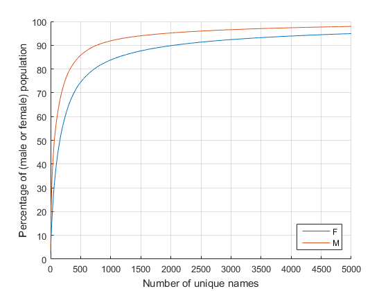
And now I can make a grouped plot by using splitapply with plot as my function. Again, plot isn't the kind of function you'd normally use with splitapply, but does it work? Yes! (Just remember to hold on so that the repeated calls to plot don't overwrite each other.)
figure
hold on
splitapply(@plot,names.CumulativeDist,gender);

legend(categories(names.Gender),'Location','southeast')
axis([0 5000 0 100])
xlabel('Number of unique names')
ylabel('Percentage of (male or female) population')
grid on
hold off

From this you can see that about 3/4 of girls (in the U.S. since 1880) have shared the set of the most popular 500 names. And a little over 85% of boys have shared the same number. Let's zoom in...
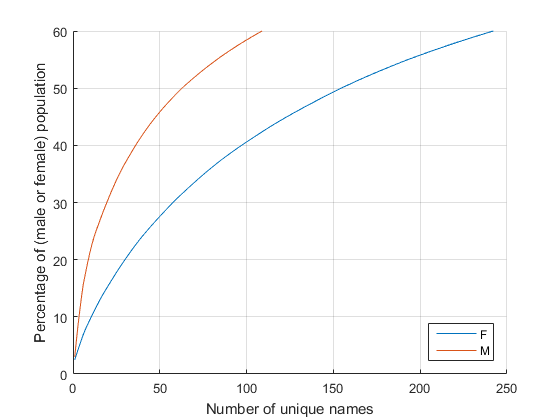
axis([0 250 0 60])

Only about 60 names are needed to address half the men in the U.S! With a little creativity, I can probably get the exact number...
qntl = @(x) find(x >= 50,1,'first');
splitapply(qntl,names.CumulativeDist,gender)
ans =
   155
    63
This splitapply function is quite useful! Let's find the 25% quartile number.
qntl = @(x) find(x >= 25,1,'first');
splitapply(qntl,names.CumulativeDist,gender)
ans =
    43
    14
How about that? One in every four males you know (in the U.S., ignoring changing trends over time) has one of these 14 names:
boys = names.Name(names.Gender == 'M');
disp(boys(1:14,:))
     James
     John
     Robert
     Michael
     William
     David
     Joseph
     Richard
     Charles
     Thomas
     Christopher
     Daniel
     Matthew
     George
And there I am on that list. Along with my brother, father, and grandfathers. Oh well. At least I have a weird last name to make up for our lack of imagination!
Interestingly, girls' names show a greater diversity. I don't know why that might be or what (if anything) it means, but it does align with my highly unscientific anecdotal evidence from parents that there are more "good" options when choosing names for girls than boys.
Where will findgroups and splitapply take you?
There is an old saying that if all you have is a hammer, everything looks like a nail. Maybe I'm guilty of falling into that trap, but I prefer to think of it as seeing just what this new "hammer" thing can do. And in this case, it looks like a pretty handy tool. From conversations about baby names I've already found some interesting applications of findgroups and splitapply. In return they've led me to some intriguing findings about how boys and girls names are distributed.
How about you? Have you done some analysis where splitapply might have helped? Let us know here.


Comments
To leave a comment, please click here to sign in to your MathWorks Account or create a new one.