MATLAB is Satisfying

Today's guest post comes from Sean de Wolski, one of Loren's fellow Application Engineers. You might recognize him from MATLAB answers and the pick of the week blog!

Contents

I manned the MathWorks booth one of the days last week at the annual SIAM conference in Boston MA. The keynote speaker that day was Donald Knuth who was there to discuss satisfiability and the latest chapter of his book, "The Art of Computer Programming".

At the beginning of the session, he provided a satisfiability puzzle, similar to a Sudoku puzzle, for those in the audience to do.

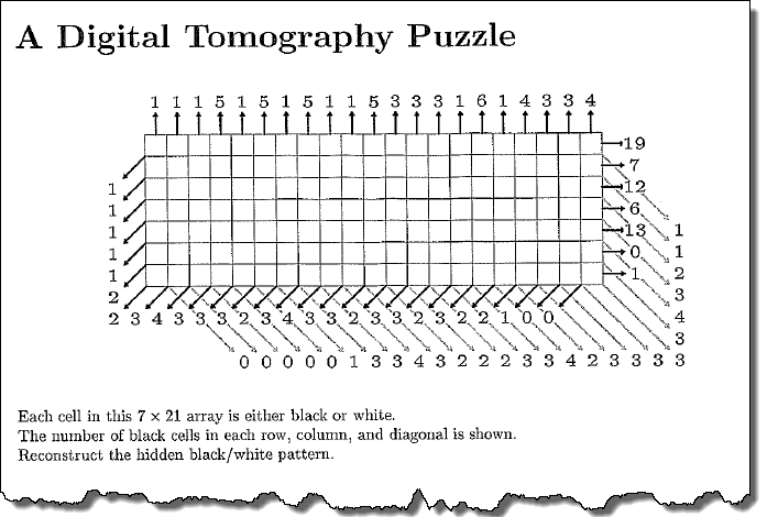
I figured, why not solve it with MATLAB?

NOTE If you would like to solve the puzzle by hand don't scroll down!

Set Up

First, let's define some useful information about the sizes. By making these variables, and parameterizing everything else this approach will scale to similar puzzles of any size!

m = 7; % rows
n = 21; % columns
nv = m*n; % number of elements

Bounds and Integer Constraints

We will solve this as a binary integer programming problem using intlinprog. The variables names used will be the same from the documentation. Each square will have a value of one or zero. Since the solver expects to work for a column vector, we will be turning the matrix into a vector columnwise, the equivalent of m(:).

Lower and upper bounds.

lb = zeros(1,nv);
ub = ones(1,nv);

All variables are binary and therefore integer constrained.

intcon = 1:nv;

This is a feasibility problem so f can be anything.

f = zeros(nv,1);

Equality Constraints

The equality constraints are the hardest part. We need to ensure that each column, row, diagonal, and anti-diagonal sum to the number shown.

The sum of each dimension, given to us by the puzzle, is the beq constraint.

The Aeq coefficient constraint will be a binary matrix with a specific sparsity pattern.

Row and Column

For the row and column coefficient matrix, Aeq, we need to replicate an identity matrix the size of the other dimension by block for rows and by element for columns. It will be replicated x times, where x is the size of the dimension.

Aeqrows = repmat(eye(m),1,n);
beqrows = [19;7;12;6;13;0;1];

Aeqcols = repelem(eye(n),1,m);
beqcols = [1 1 1 5 1 5 1 5 1 1 5 3 3 3 1 6 1 4 3 3 4]';

View the sparsity pattern of the constraints and what they sum to.

subplot(1,10,1:4)
imagesc(Aeqcols)
xlabel('Column Coefficients')
title('Column equality constraints')
subplot(1,10,5)
imagesc(beqcols)
xlabel('Column Sum')

subplot(1,10,6:9)
imagesc(Aeqrows)
xlabel('Row Coefficients')
title('Row equality constraints')
subplot(1,10,10)
imagesc(beqrows)
xlabel('Row sum')

Diagonal and Antidiagonal

We will use the same algorithm for the diagonal and antidiagonal pieces.

The beq matrices will be the sums, starting on the left.

The Aeq matrices will be built using diag to extract diagonals from matrix of linear indices. This means each value in the matrix idx will be it's linear index.

For the antidiagonals, we'll just flip beq and idx but use the same approach.

A for-loop will then traverse every diagonal, and turn the corresponding indices in the Aeq coefficient matrices to true.

Aeqdiag = zeros(m+n-1,nv);
Aeqantidiag = Aeqdiag;
beqdiag = [0 0 0 0 0 1 3 3 4 3 2 2 2 3 3 4 2 3 3 3 3 3 4 3 2 1 1].';
beqantidiag = flip([1 1 1 1 1 2 2 3 4 3 3 3 2 3 4 3 3 2 3 3 2 3 2 2 1 0 0]).';

idx = reshape(1:nv,m,n);
antidx = flip(idx,2);
for ii = -(m-1):n-1
    Aeqdiag(ii+m,diag(idx,ii)) = 1;
    Aeqantidiag(ii+m,diag(antidx,ii)) = 1;
end

View the sparsity pattern of the constraints and what they sum to.

subplot(1,10,1:4)
imagesc(Aeqdiag)
xlabel('Diag Coeff')
title('Diagonal equality constraints')
subplot(1,10,5)
imagesc(beqdiag)
xlabel('Diag Sum')

subplot(1,10,6:9)
imagesc(Aeqantidiag)
xlabel('Antidiag Coeff')
title('Antidiagonal equality constraints')
subplot(1,10,10)
imagesc(beqantidiag)
xlabel('Antidiag Sum')

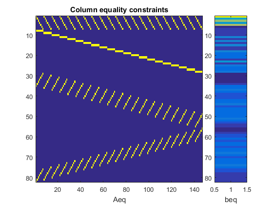
The equality constraints we've built are all independent from one another, we just need to concatenate them together in an arbitrary order to build the full equality constraints.

Aeq = [Aeqrows;Aeqcols;Aeqdiag;Aeqantidiag];
beq = [beqrows;beqcols;beqdiag;beqantidiag];

View.

figure
subplot(1,5,1:4)
imagesc(Aeq)
xlabel('Aeq')
title('Column equality constraints')
subplot(1,5,5)
imagesc(beq)
xlabel('beq')

Solve!

Call the intlinprog solver.

x = intlinprog(f,intcon,[],[],Aeq,beq,lb,ub);

LP:                Optimal objective value is 0.000000.                                             


Optimal solution found.

Intlinprog stopped at the root node because the objective value is within a gap
tolerance of the optimal value, options.AbsoluteGapTolerance = 0 (the default
value). The intcon variables are integer within tolerance,
options.IntegerTolerance = 1e-05 (the default value).

View the Result

x is a vector,so we'll need to undo the m(:) operation from above to reshape it to be the grid size before viewing.

xi = reshape(x,m,n);

figure
imagesc(xi)
axis tight equal off

Ahh, I see what's going on. Let's make it prettier.

s = surf([rot90(xi,2); zeros(1,n)]);
view(0, -90)
axis tight equal off
s.EdgeColor = [0.8 0.8 0.8];

Any comments? Let us know here.

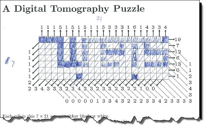
And just for completeness, Christine Tobler, who was sitting next to me did solve it first by hand.

Get the MATLAB code

Published with MATLAB® R2016a