Introducing String Arrays
Toshi is back for today's guest post. You may have seen Toshi's earlier posts about text analytics and he often deals with text in his data analysis. So he is very excited about new string arrays in R2016b.

One of the new features I love in R2016b is string arrays, which give you a new way to handle text in MATLAB in addition to the familiar character arrays and cell arrays of character vectors. String arrays are most helpful when dealing with text in your data. In today's post I walk through some practical examples with text data to demonstrate how to use string arrays.
Contents
- Analyzing Baby Name Trends
- String Concatenation
- Combine Files to Create a Single Table
- String Comparison
- Memory Use and Performance of String Arrays vs. Cell Arrays
- Data Wrangling Example
- Fixing Typos or Inconsistent Labeling
- Find and Convert Substrings
- Tokenization
- Document Term Frequency Matrix
- Non-English Text
- Summary
Analyzing Baby Name Trends
Let's play with strings using the baby names dataset from Social Security Administration. The data is stored in separate text files by year of birth from 1880 to 2015. Let's begin by previewing one of them.
if ~isdir('names')                                          % if |names| folder doesn't exist
    url = 'https://www.ssa.gov/oact/babynames/names.zip';   % url of the zipped data file
    unzip(url,'names')                                      % download and unzip data into |names| folder
end
tbl1880 = readtable('names/yob1880.txt');                   % read the first file
vars = {'name','sex','births'};                             % column names
tbl1880.Properties.VariableNames = vars;                    % add column names
disp(tbl1880(1:5,:))                                        % preview 5 rows
       name        sex    births
    ___________    ___    ______
    'Mary'         'F'    7065
    'Anna'         'F'    2604
    'Emma'         'F'    2003
    'Elizabeth'    'F'    1939
    'Minnie'       'F'    1746
String Concatenation
Rather than loading each file into a separate table, we would like to create a single table that spans all the years available. The files are named with a convention: 'yob' + year + '.txt', which we can use to generate the file paths. With a string array, we can take advantage of array expansion to generate the list of filenames.
years = 1880:2015;                                          % vector of years in double
filepaths = string('names/yob') + years + '.txt';           % concatenate string with numbers
filepaths(1:3)                                              % indexing into the first 3 elements
ans =
  1×3 string array
    "names/yob1880.txt"    "names/yob1881.txt"    "names/yob1882.txt"
Combine Files to Create a Single Table
Let's create a single table that spans all the years available. Note that we need to use char to convert the individual filename strings to character vectors for use with readtable. We'll set the readtable parameter TextType to 'string' so that the text data is read into the table as string arrays. When you preview the first five rows, notice that text is surrounded by double quotes rather than single quotes, which indicates they are represented as string arrays.
names = cell(length(years), 1);                             % accumulator
for ii = 1:length(years)                                    % for each year
    names{ii} = readtable(char(filepaths(ii)), ...          % read individual files
        'ReadVariableNames', false, ...                     % into separate tables
        'TextType','string');                               % with text in string arrays
    names{ii}.Properties.VariableNames = vars;              % add column names
    names{ii}.year = repmat(years(ii), ...                  % add |year| column
        height(names{ii}), 1);
end
names = vertcat(names{:});                                  % concatenate tables
disp(names(1:5,:))                                          % preview 5 rows
       name        sex    births    year
    ___________    ___    ______    ____
    "Mary"         "F"    7065      1880
    "Anna"         "F"    2604      1880
    "Emma"         "F"    2003      1880
    "Elizabeth"    "F"    1939      1880
    "Minnie"       "F"    1746      1880
String Comparison
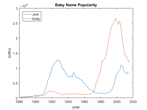
Let's plot how the popularity of the names 'Jack' and 'Emily' have changed over time. With string arrays, you can simply use the == operator for comparison. This makes our code clearer as compared to using strcmp. We can observe that Emily has seen a surge of popularity in recent years and Jack is staging a comeback.
Jack = names(names.name == 'Jack', :);                      % rows named 'Jack' only
Emily = names(names.name == 'Emily', :);                    % rows named 'Emily' only
Emily = Emily(Emily.sex == 'F', :);                         % just girls
Jack = Jack(Jack.sex == 'M', :);                            % just boys
figure                                                      % new figure
plot(Jack.year, Jack.births);                               % plot Jack
hold on                                                     % don't overwrite
plot(Emily.year, Emily.births);                             % plot Emily
hold off                                                    % enable overwrite
title('Baby Name Popularity');                              % add title
xlabel('year'); ylabel('births');                           % add axis labels
legend('Jack', 'Emily', 'Location', 'NorthWest')            % add legend

Memory Use and Performance of String Arrays vs. Cell Arrays
Let's consider the impact string arrays have on memory usage.
namesString = names.name;                                   % this is string
namesCellAr = cellstr(namesString);                         % convert to cellstr
whos('namesString', 'namesCellAr')                          % check size and type
  Name                   Size                Bytes  Class     Attributes

  namesCellAr      1858689x1             231124058  cell
  namesString      1858689x1             120288006  string
The string array uses about half the memory of the cell array of character vectors in this case. The memory savings depends on the array data and size and is pronounced for arrays with many elements like this one.
In most cases, you can also achieve better performance when you use string arrays with new string manipulation methods. replace is a new string method which you can often use in place of strrep for replacing substrings of text. Notice the performance difference:
tic, strrep(namesCellAr,'Joey','Joe'); toc,                 % time strrep operation
tic, replace(namesString,'Joey','Joe'); toc,                % time replace operation
Elapsed time is 0.807283 seconds.
Elapsed time is 0.409385 seconds.
Data Wrangling Example
School of Data hosts GRAIN landgrab data collected by an NGO. It is a typical messy dataset that requires some cleaning.
if exist('grain.xls', 'file') ~= 2                          % if file doesn't exist
    url = 'https://commondatastorage.googleapis.com/ckannet-storage/2012-08-14T085537/GRAIN---Land-grab-deals---Jan-2012.xls';
    websave('grain.xls', url);                              % save file from the web
end
data = readtable('grain.xls', 'Range', 'A2:I417', ...       % load data from file
    'ReadVariableNames', false, 'TextType', 'string');
Fixing Typos or Inconsistent Labeling
One common data cleaning issue is dealing with typos or inconsistent labeling. Let's take an example from the table column Landgrabber, which contains entity names. You see two spelling variants for the same entity.
entities = string(data.(2));                               % entity as a string array
entities([18,350])                                         % subset
ans =
  2×1 string array
    "Almarai Co"
    "Almarai Co."
String arrays provide a variety of methods for efficiently manipulating text values, particularly when working with lots of text data. Here we'll use endsWith to find the names missing a period after 'Co'.
isCo = endsWith(entities,'Co');                            % find all that ends with 'Co'
entities(isCo) = entities(isCo) + '.';                     % add period
entities(isCo)                                             % check the result
ans =
  8×1 string array
    "Almarai Co."
    "Shaanxi Kingbull Livestock Co."
    "Foras International Investment Co."
    "Foras International Investment Co."
    "Foras International Investment Co."
    "Foras International Investment Co."
    "Foras International Investment Co."
    "Foras International Investment Co."
Find and Convert Substrings
The table column ProjectedInvestment contains dollar amounts in both millions and billions as text. Let's use the contains methods to find where millions and billions are used.
investment = data.(7);                                      % subset a column
investment(1:5)                                             % preview the first 5 rows
isMillion = contains(investment,'million');                 % find rows that contain substring
isBillion = contains(investment,'billion');                 % find rows that contain substring
ans =
  5×1 string array
    ""
    "US$77 million"
    ""
    "US$30-35 million"
    "US$200 million"
Let's use regexp to extract numbers. When a range like 'US$30-35 million' is given, we will use the first number. String arrays work with regular expressions just like cell arrays of character vectors. Lastly, we'll remove commas with replace.
pattern = '\d+\.?,?\d*';                                    % regex pattern
num = regexp(investment, pattern, 'match', 'once');         % extract first matches
num = replace(num, ',', '');                                % remove commans
num(1:5)                                                    % preview the first 5 rows
ans =
  5×1 string array
    <missing>
    "77"
    <missing>
    "30"
    "200"
You notice that this regular expression call created <missing> values when it didn't find matches. This is the string equivalent to NaN in numeric arrays. We don't need to treat these missing values differently here since these missing values will convert to NaN when we cast the value to double, which is what we want. After casing to double, we'll adjust the scale of each value to be in the millions or billions.
num = double(num);                                          % convert to double
num(isMillion) = num(isMillion) * 10^5;                     % adjust the unit
num(isBillion) = num(isBillion) * 10^8;                     % adjust the unit
num(1:5)                                                    % preview the first 5 rows
ans =
         NaN
     7700000
         NaN
     3000000
    20000000
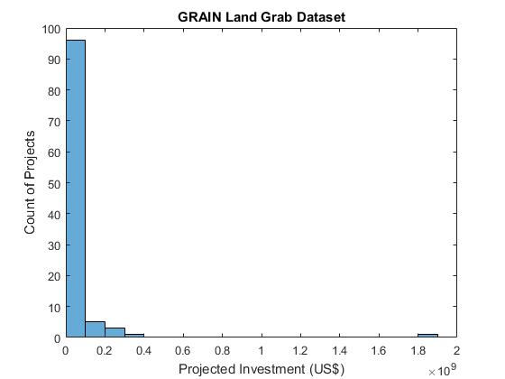
Now let's plot the result as histogram.
figure                                                      % new figure
histogram(num)                                              % plot histogram
xlabel('Projected Investment (US$)')                        % add x-axis label
ylabel('Count of Projects')                                 % add y-axis label
title('GRAIN Land Grab Dataset')                            % add title

Tokenization
One of the common approaches in text analytics is to count the occurrences of words. We can tokenize the whole string array and generate a list of unique words as a dictionary. Check out how string arrays seamlessly work with familiar functions like lower, ismember or unique. We can also use new functions like erase. To standardize the word form we will deal with things like plurals and conjugations using the legacy Porter Stemmer code. It takes character vectors, so we'll need to convert strings to character vectors with char when we use it.
summary = data.(9);                                         % extract Summary
delimiters = {' ',',','.','-','"','%','(',')','&','/','$'}; % characters to split with
stopwordsURL ='http://www.textfixer.com/resources/common-english-words.txt';
stopWords = urlread(stopwordsURL);                          % read stop words
stopWords = split(string(stopWords),',');                   % split stop words
stemmer_url = 'http://tartarus.org/martin/PorterStemmer/matlab.txt';
if exist('porterStemmer.m', 'file') ~= 2                    % if file doesn't exist
    websave('porterStemmer.txt',stemmer_url);               % save file from the web
    movefile('porterStemmer.txt','porterStemmer.m','f')     % rename file
end
tokens = cell(size(summary));                               % cell arrray as accumulator
for ii = 1:length(summary)                                  % for each row in summary
    s = split(summary(ii), delimiters)';                    % split content by delimiters
    s = lower(s);                                           % use lowercase
    s = regexprep(s, '[0-9]+','');                          % remove numbers
    s(s == '') = [];                                        % remove empty strings
    s(ismember(s, stopWords)) = [];                         % remove stop words
    s = erase(s,'''s');                                     % remove possessive s
    for jj = 1:length(s)                                    % for each word
        s(jj) = porterStemmer(char(s(jj)));                 % get the word stem
    end
    tokens{ii} = s;                                         % add to the accumulator
end
dict = unique([tokens{:}]);                                 % dictionary of unique words
Document Term Frequency Matrix
Now we can count the number of occurrences of all words in the dictionary across all rows by creating the document term frequency matrix.
DTM = zeros(length(tokens),length(dict));                   % accumulator
for ii = 1:length(tokens)                                   % loop over tokens
    [words,~,idx] = unique(tokens{ii});                     % get uniqe words
    wcounts = accumarray(idx, 1);                           % get word counts
    cols = ismember(dict, words);                           % find cols for words
    DTM(ii,cols) = wcounts;                                 % unpdate dtm with word counts
end
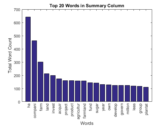
Let's plot the frequency of the top 20 stemmed words. We can do fancier analysis with document term frequency matrix, such as text classification, sentiment analysis and text mining.
Check out my post Can You Find Love through Text Analytics?, Analyzing Twitter with MATLAB and Text Mining Shakespeare with MATLAB and Text Mining Machine Learning Research Papers with MATLAB for more details.
[wc, ii] = sort(sum(DTM), 'descend');                       % sort dtm by word count
figure                                                      % new figure
bar(wc(1:20))                                               % plot the top 20
ax = gca;                                                   % get current axes hande
ax.XTick = 1:20;                                            % set x axis tick
ax.XTickLabel = dict(ii(1:20));                             % label x axis tick
ax.XTickLabelRotation = 90;                                 % rotate x axis tick label
xlim([0 21])                                                % set x axis limits
xlabel('Words')                                             % add x axis label
ylabel('Total Word Count')                                  % add y axis label
title('Top 20 Words in Summary Column')                     % add title

Non-English Text
Let's not forget that we often deal with non-English text, especially if the data source is from the internet such as Twitter. Let's load the sample data from an Excel file that contains text in French, Italian, German, Spanish, Chinese, Japanese and Korean (so-called FIGS and CJK text). Chinese and Japanese words for "string" seem to share a common character. Let's confirm this using contains we saw earlier.
[~, ~, nonenglish] = xlsread('non_english.xlsx');           % load text from Excel
nonenglish = string(nonenglish);                            % convert to string
disp(nonenglish(:,[1,6:7]))                                 % preview 3 columns
cj_string = nonenglish(3,6:7);                              % "string" in Chinese and Japanese
contains(cj_string(1), cj_string{2}(2))                     % is Japanese char in Chinese text?
    "English"                 "Chinese"           "Japanese"
    "English"                 "中文"              "日本語"
    "string"                  "字符串"             "文字列"
    "Do you speak MATLAB?"    "你会说MATLAB吗?"    " あなたはMATLABを話..."
ans =
  logical
   1
Korean, like English, uses white space to separate words. We can use that to split string into tokens.
kr_string = nonenglish(4,8);                                % "Do you speak MATLAB" in Korean
split(kr_string)                                            % split string by whitespace
ans =
  3×1 string array
    "당신은"
    "MATLAB을"
    "말합니까?"
For languages that do not use whitespace characters to separate words, we would need to use specialized tools to split words, such as Japanese Morphological Analyzer MeCab discussed in my post Can You Find Love through Text Analytics? and you can find more details about how to use it with MATLAB in this File Exchange entry.
Summary
String arrays are a useful new data type for working with text data. String arrays behave more like numeric arrays, can make code more readable, and are more efficient for storing text data and performing string manipulations.
Try using string arrays with your text data instead of cell arrays of character vectors. Doing so will make your code clearer and concise especially if you take advantage of new functions. You can also avoid the need for cellfun with function handles and the UniformOutput flag that cell arrays of character vectors often require.
Obviously I am pretty excited about string arrays. Play with string arrays and let us know what you think here!
- Category:
- New Feature,
- Strings


Comments
To leave a comment, please click here to sign in to your MathWorks Account or create a new one.