Symbolic Analysis of the Port Passing Problem

Contents

Introduction

Hopefully you recall the recent post where we used a monte-carlo technique to simulate an infinitely-stocked port decanter passing around a table of N people (always starting at position 0), moving with probability p to the left and q to the right, only stopping when everyone at the table had received some port. Those simulations seemed to show that simple analytic solutions to expected path lengths might be possible and today, I'll show you what I managed to prove.

In the last post we decided that the functions we wanted to find are

Gambler's Ruin

Thanks to my colleague Rick Amos, we have a starting point for thinking about an analytical solution. He pointed out that our port passing problem was very similar to the random walk process Gambler's Ruin, in which the gambler starts out with some stake (k) and wins another unit of that stake with probability p (or loses with probability 1-p). The game continues until the gambler has either lost all the money, or has a total of N. The major difference is that in Gambler's Ruin there are two different end conditions (winning with N or losing with 0).

To enable us to attack the port passing problem, I'll need to quote two results from Gambler's Ruin. You can find derivations of these results in the associated files on File Exchange (see the files BiasedGamblersRuin and UnbiasedGamblersRuin). The first result allows us to answer the question: "what is the probability, given that we are currently at position S, of arriving at position A before arriving at position B?". In terms of Gambler's Ruin this is the same as starting with stake $k=S-B$ and finishing with $N=A-B$. To make some of the equations simpler I'll use $q=1-p$, and note we assume $A<S<B \mbox{ or } B<S<A$.

$$pSAB=\left\lbrace \begin{array}{cc}\frac{k}{N} & p=q=\frac{1}{2}\\\frac{1-r^k}{1-r^N} & p\ne q\mbox{ and } r=\frac{q}{p}\end{array}\right.$$

Similarly, we also need to answer: "what is the expected number of passes (starting at S) to arrive at position A before arriving at position B?".

$$eSAB=\left\lbrace \begin{array}{cc}\frac{N^2-k^2}{3} & p=q=\frac{1}{2}\\\frac{1+r}{1-r}(N(\frac{2}{1-r^N }-1)-k(\frac{2}{{1-r}^k }-1)) & p\ne q\end{array}\right.$$

Note how each result has a different expression for the biased and unbiased case? Below we will run through the biased case (which has more complexity). Exactly the same code could be run with the unbiased case and the correct result obtained - if you are interested simply change pToUse below back to 0.5 and execute.

syms pSAB(S,A,B) eSAB(S,A,B) p q k N

pToUse = 0.55;
assume(p == pToUse);

% Define the functions for k and N in terms of S, A, and B.
k(S,A,B) = S-B;
N(S,A,B) = A-B;

if pToUse == 0.5
    pSAB(S,A,B) = k/N;
    eSAB(S,A,B) = (N^2 - k^2)/3;
else
    % In the biased case we will use r rather than p in the equations
    syms r
    assume(r ~= 1);

    pSAB(S,A,B) = (1-r^k)/(1-r^N);
    eSAB(S,A,B) = (1+r)/(1-r) * (N*(2/(1-r^N)-1) - k*(2/(1-r^k)-1));
end

To allow us to talk about the general case where position k is the last to receive the port around a table of size N we will use position L to refer to a position one to the right of k and R to one to the left of k (note the use of modulo arithmetic to ensure $k-N<R \le 0 \le L < k$ and that the direction left is defined as an increase in position number, and right is a decrease in position number).

syms L R N k
L = k-1;
R = k+1-N;

Calculating the probability that position k is last

For position k to be last we either need the port to move from the starting position 0 to L and then to R, or move from 0 to R and then L. This probability is given by

$$p_k = pSAB(0,L,R) * pSAB(L,R,k) + pSAB(0,R,L) * pSAB(R,L,k)$$

p0L = pSAB(0, L, R);
p0R = pSAB(0, R, L);
pLR = pSAB(L, R, k);
pRL = pSAB(R, L, k-N);
p0LR = p0L*pLR;
p0RL = p0R*pRL;

pk = simplify(p0LR + p0RL)

pk =
-(r^N*(r - 1))/(r^k*(r - r^N))

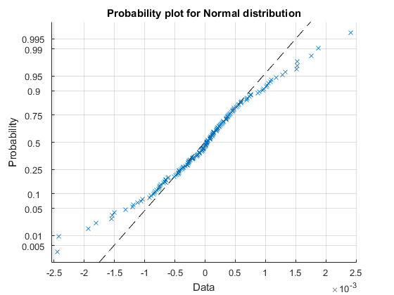
In the previous blog post we showed that for the unbiased case this result was independent of position k, but in the biased case the position around the table affects the last probability. Let's look at the residuals from some simulations to check if this is correct (the portPassingSimulation code is available here).

p = pToUse;
N = 17;
k = 1:N-1;
nSims = 1e5;
residuals = NaN(10,N-1);
expected = double(subs(pk, {'r' 'N' 'k'}, {(1-p)/p, N, k}));
% Simulate 10 times passing around a table of 17
parfor ii = 1:10
    last = portPassingSimulation(nSims, N, p);
    % Group simulations into k (1:N-1) bins and normalize by number of simulations
    lastProb = hist(last, k)/nSims;
    residuals(ii, :) = lastProb - expected;
end
% Are the residuals normally distributed?
probplot('normal', residuals(:))
grid on

We can see that the residuals from the simulation are roughly normally distributed (some tail points are not quite normal) but there isn't any bias from the expected results (because the mean of the residuals is close to zero).

meanR = mean(residuals(:))

meanR =
   7.5894e-20

What routes do we need to consider to compute the expected path length?

To compute the expected path length, we are going to have to consider all possible paths that finally end with position k, work out the probability with which each path occurs and multiply by the expected length of that path. Fortunately, whilst there are infinitely many possible paths we can decompose the problem into just 2 that relate directly to Gambler's Ruin. These are the L route and R route as specified by

The alternative route R (which is basically the inverse of route L) is

The expected lengths of each of these parts of the path are

syms k N
E0L  = eSAB(0, L, R);
E0R  = eSAB(0, R, L);

ELR  = eSAB(L, R, k);
ERL  = eSAB(R, L, k-N);

ERk  = eSAB(R, k-N, k);
ELk  = eSAB(L, k, k-N);

ERLk = eSAB(R, k, k-N);
ELRk = eSAB(L, k-N, k);

It is interesting to note that the expected path length eSAB is symmetric with respect to swapping the variables p and q. We can see this in the above equations as ELR==ERL, ERk==ELk and ERLk==ELRk

simplify(ELR  == ERL)
simplify(ERk  == ELk)
simplify(ELRk == ERLk)

ans =
TRUE
ans =
TRUE
ans =
TRUE

To combine the parts of route L and route R where there is a choice we need to include the probabilities of undertaking part 3 and 4 of L and part 3 and 4 of R. These are simply the probabilities of those paths in Gambler's Ruin.

pRk  = pSAB(R, k-N, k);
pLk  = pSAB(L, k, k-N);

pRLk = pSAB(R, k, k-N);
pLRk = pSAB(L, k-N, k);

So finally we can combine these parts for our two routes. EL is the expected path for route L and ER the expected path length for route R.

EL = E0L + ELR + pRk.*ERk + pRLk.*ERLk;
ER = E0R + ERL + pLk.*ELk + pLRk.*ELRk

ER =
((1/r - 1)*(r + 1)*(2/(1/r - 1) - N*(2/(1/r^N - 1) + 1) + 1))/((r - 1)*(1/r^N - 1)) - (((2/(r^(2 - N) - 1) + 1)*(N - 2) - (2/(r^(1 - k) - 1) + 1)*(k - 1))*(r + 1))/(r - 1) - ((r + 1)*(2/(r - 1) - (N - 1)*(2/(r^(N - 1) - 1) + 1) + 1))/(r - 1) - (((N - 1)*(2/(r^(N - 1) - 1) + 1) - N*(2/(r^N - 1) + 1))*(r + 1)*(r^(N - 1) - 1))/((r^N - 1)*(r - 1))

I've only printed one result out simply to show that at the moment this looks pretty complicated! Hopefully this is going to get simpler some way down the line!

Probability that the port takes route L or R

To be able to compute the overall expected path we also need to know the probability that the port takes route L or R, since

$$E_k = p_L E_L + p_R E_R$$

Fortunately, we already have the components to compute these probabilities from the analysis of finish position probabilities. The probability the we take route L is just the probability of from 0 to L to R divided by the probability that k is last. Similarly, for the route R.

pL = simplify(p0L*pLR/pk)
pR = simplify(p0R*pRL/pk)

pL =
(r^N - r^(k + 1))/(r^N - r^2)
pR =
-(r*(r - r^k))/(r^N - r^2)

Calculating the expected path length when k is last

With all these results in place we can compute the expected length by adding the two possible path lengths times their probabilities.

Ek = simplify(pL.*EL + pR.*ER, 400)

Ek =
(2*(2*N - k - 3*r^N + N*r^N - N*r^k + k*r^N + 1))/((r^N - 1)*(r - 1)) - (k - 2*N + N*r^N + N*r^k - k*r^N)/(r^N - 1) - 4/(r - 1)^2 - (2*r^N*(r^N + 1)*(N - 1))/((r - r^N)*(r^N - 1))

Does this agree with simulation?

We can look to see how well Ek agrees with the simulated data by running the simulation and computing the mean number of passes for each finishing position. As we saw in the previous blog post, a simple way to look at the mean number of passes for each last position is by using varfun for a table, with a grouping variable.

p = pToUse;
N = 17;
k = 1:N-1;
[last,nPass] = portPassingSimulation(1e6, N, p);
t = varfun(@mean, table(last, nPass), ...
    'GroupingVariable', 'last')

t = 
    last    GroupCount    mean_nPass
    ____    __________    __________
     1            9291    95.262    
     2           11379    111.75    
     3           13888    123.74    
     4           17016    130.06    
     5           20845    135.69    
     6           25541    136.47    
     7           31030    136.05    
     8           38271     133.8    
     9           46659    130.33    
    10           56701    125.85    
    11           69383    119.94    
    12           84602    112.84    
    13        1.04e+05    106.39    
    14      1.2629e+05    98.765    
    15      1.5536e+05    90.384    
    16      1.8975e+05    82.086    

Plotting these against the analytical results gives

cMean = double(subs(Ek, {'r' 'N' 'k'}, {(1-p)/p N k}));
plot(t.last, t.mean_nPass, 'ro');
hold on
plot(k, cMean, '.-')
grid on
hold off
title 'Simulated vs expected mean number of passes'
xlabel 'Position port received last at the table'
ylabel 'Mean number of passes to reach last position at table'
legend('Simulated results', 'Expected result')

And lastly the difference in the mean and expected mean is almost zero

mean(cMean(:) - t.mean_nPass(:))

ans =
    -0.041108

The average of the residuals is close to zero showing the simulated data are in agreement with the expression.

What is the mean number of passes needed for a table of size N?

Having deduced the expected number of passes needed when the last position is k, we can now, finally, compute the expected path length for the table of size N because we can simply sum the expected path for each of the possible k positions times the probability that position k is the last.

$$E_N =\sum_{k=1}^{N-1} p_k E_k$$

syms k N r
EN = simplify(symsum(pk*Ek, k, 1, N-1), 1000)

EN =
(N^2*(r + 1))/((r^N - 1)*(r - 1)) - ((r + 1)*(N + r - N*r))/(r - 1)^2 + (r*(N - 1)^2*(r + 1))/((r - r^N)*(r - 1))

Thankfully this looks a lot simpler than some of the other results earlier.

Check against a known analytical solution

Before continuing we can check this result in a couple of ways. Firstly, let's check specifically against the N==3 case where we already know the analytic solution (see SymbolicAnalysisFor3People.mlx)

$$E_3 =\frac{3}{q^2 -q+1}-1$$

Substituting in a value for N and equation for r

E3 = simplify(subs(EN, {N, r}, {3 q/(1-q)}), 400)

E3 =
3/(q^2 - q + 1) - 1

Alternatively, we can check the results against some simulations for different values of N

p = pToUse;
tableSize = 5:3:37;
sim = NaN(size(tableSize));
parfor ii = 1:numel(tableSize)
    N = tableSize(ii);
    [~,nPass] = portPassingSimulation(1e5, N, p);
    sim(ii) = mean(nPass);
end
plot(tableSize, sim, 'ro')
grid on
hold on
N = min(tableSize):max(tableSize);
expected = double(subs(EN, {'r' 'N'}, {(1-p)/p N}));
plot(N, expected);
hold off
title 'Expected passes to finish random walk'
xlabel 'Number of people at the table'
ylabel 'Number of passes'
legend('Simulated results', 'Expected result', 'Location', 'N')

Writing the biased and unbiased results out in full, we get

$$E_N =\left\lbrace \begin{array}{cc}\frac{N(N-1)}{2} & p=q=\frac{1}{2}\\\frac{r+1}{r-1}(\frac{N^2}{r^N -1}-\frac{{(N-1)}^2 }{r^{N-1} -1}+\frac{Nr-N-r}{r-1})& p\ne q\end{array}\right.$$

Written this way, it is quite complicated, but there is a symmetry to it. A term in N, the same term in N-1 and another term. All-in-all distinctly simpler than ER that I printed out further up the page. And with that we have produced analytic solutions for all the values we wanted to investigate - perhaps it is now time to pass the port!

And finally

Manipulation of the fairly complicated algebraic expression that resulted from joining all the expected paths with probabilities together was something I thought would be really hard when done by hand. Yet I think you will agree using the Symbolic Math Toolbox has made it tractable. I'm also impressed with its ability to solve recurrence relationships (see the associated files that prove the initial definitions of pSAB and eSAB).

From the article it might look like I've done all the work here myself, so I'd like to thank both Rick Amos (MathWorks) and Barnaby Martin (Durham University) for helping out with many of the details.

Having seen these related blog posts, what problems might you now attack using simulation to guide your mathematical approach? Can you see opportunities to bring statistics and symbolic manipulation together? Let me know here.

Get the MATLAB code

Published with MATLAB® R2016b