
Optimizing a Structural Design
Today you'll see a new demonstration of applying optimization techniques. Today's guest is Takafumi Ohbiraki. This demonstration was part of the contents of the MATLAB EXPO which was held in Tokyo last year (2016).
Contents
- Design of an umbrella hook
- FEM model (Using Partial Differential Equation (PDE) Toolbox)
- Process of Optimization
- Design of Experiments (DOE) (Taguchi design)
- Calculation with setting parameters for L18
- Factor Effect Chart
- S/N ratio
- Output
- Optimization using patternsearch solver
- Optimization using ga solver
- Multi-objective optimization using the gamultiobj solver
- Conclusion
Optimization is a universal topic in both engineering and data science. It is a technology with high needs. Speaking of optimization in engineering, parameter estimation is often performed on a model showing a physical phenomenon.
Generally, when expressing a physical phenomenon by a model, MATLAB has functions of ordinary differential equations and partial differential equations,and performs simulation. For example, since the problem of heat conduction can be represented by parabolic partial differential equations on the second floor, it is possible to simulate with the function pdepe.
In reality, it is often difficult to convert a physical phenomenon into a closed-form mathematical formula. So it is common to utilize a modeling tool to convert the problem into a mathematical model for analysis.
At this time, we will introduce how to optimize the design by using Partial Differential Equation Toolbox and Optimization Toolbox with an example of structural analysis.
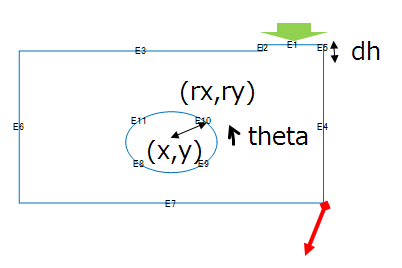
Design of an umbrella hook
A cool umbrella hook is always seen in Japanese public restrooms.

As a designer of an umbrella hook, we will consider how to reduce the cost by reducing the materials used for an umbrella hook. However, in order to keep the functionality of the umbrella hook, it is necessary to for the hook not to bend.
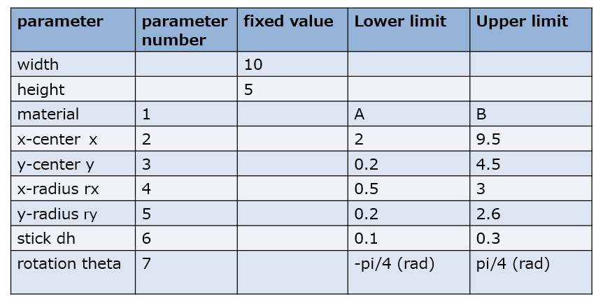
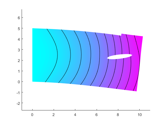
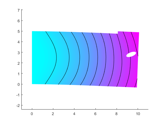
First, we define the design specifications. We consider opening an elliptical cavity in the member. The material (A or B) of the member, the coordinates (X, Y) of the ellipse, the radius of the ellipse (RX, RY), and the rotation angle of the ellipse (theta) are design parameters. The number of parameters is seven.
We will set the downward load on the tightening portion at the upper right and the fixed end at the left end. We perform an optimization with the aim of minimizing the displacement amount of the lower right point.
All parameters have the following constraints.
FEM model (Using Partial Differential Equation (PDE) Toolbox)
We create a function pdesample to actually simulate with parameters using Partial Differential Equation Toolbox (PDE Toolbox).
input: [material x-position y-position x-radius y-radius stick theta] output : strain
in = [1 5,2,1.5,1.0,0.3,0];
lh = pdesample
out = lh{1}(in)
lh =
  5×1 cell array
    @pdesample_input
    @pdesample_input_doe_sn
    @myobjfun
    @myobjfun2
    @mynoncon
out =
      0.40131
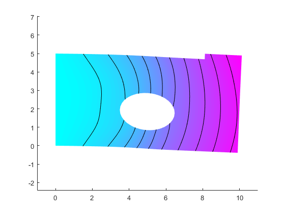
This is the initial condition.
Output is about 0.4013. We do not understand whether this result is good or bad. We will seek a good answer using optimization techniques.
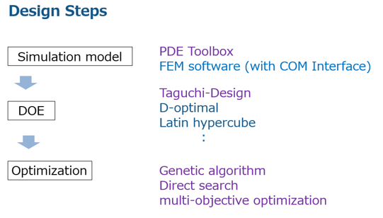
Process of Optimization
To actually perform the optimization calculation, if there are too many parameters, it takes time to reach the optimum value. This time, we will utilize a two-step optimization method that is often used in quality engineering. According to the two-step design method, first, make efforts to reduce the number of variables to be optimized by utilizing the experimental design method. In this method, we adopt the Taguchi design. The orthogonal table is uploaded to the File Exchange. In variable selection, we paid attention to the signal to noise ratio (S/N) ratio and the nominal-is-best response. In the second step, we use optimization algorithms to find good parameters.
Design of Experiments (DOE) (Taguchi design)
We will exploit which parameters should be reduced by utilizing the orthogonal array famous from the Taguchi design. In the orthogonal array of Taguchi design, there are 2 factors, 3 factors, and mixed orthogonal tables. We chose the famous L18 model for mixing both 2 factors and 3 factors.
L18 model : 18 experiments to make the combination of 8 variables efficient; one variable (material) is 2 levels , seven variables are 3 levels. The variable design created by my helper function orthogonalarray is a MATLAB table.
design = orthogonalarray('L18','Bounds',[1 2;2.0 8.0;1.0 3.0;0.5 1.9;0.2 0.9;0.1 0.3;-pi/12 pi/12;0 0],...
    'VariableNames',{'material','x','y','rx','ry','dh','theta','xxx'})
design =
  18×8 table
    material    x    y    rx      ry     dh      theta     xxx
    ________    _    _    ___    ____    ___    _______    ___
    1           2    1    0.5     0.2    0.1    -0.2618    0
    1           2    2    1.2    0.55    0.2          0    0
    1           2    3    1.9     0.9    0.3     0.2618    0
    1           5    1    0.5    0.55    0.2     0.2618    0
    1           5    2    1.2     0.9    0.3    -0.2618    0
    1           5    3    1.9     0.2    0.1          0    0
    1           8    1    1.2     0.2    0.3          0    0
    1           8    2    1.9    0.55    0.1     0.2618    0
    1           8    3    0.5     0.9    0.2    -0.2618    0
    2           2    1    1.9     0.9    0.2          0    0
    2           2    2    0.5     0.2    0.3     0.2618    0
    2           2    3    1.2    0.55    0.1    -0.2618    0
    2           5    1    1.2     0.9    0.1     0.2618    0
    2           5    2    1.9     0.2    0.2    -0.2618    0
    2           5    3    0.5    0.55    0.3          0    0
    2           8    1    1.9    0.55    0.3    -0.2618    0
    2           8    2    0.5     0.9    0.1          0    0
    2           8    3    1.2     0.2    0.2     0.2618    0
Calculation with setting parameters for L18
At experimental points, we calculate the outputs (strain) and S/N ratios.
output = zeros(18,1);
sn = zeros(18,1);

for i = 1:18
    output(i,1) = lh{1}(table2array(design(i,1:8)));
    sn(i,1) = lh{2}(table2array(design(i,1:8)));
end

results = [design table(output,sn)]
results =
  18×10 table
    material    x    y    rx      ry     dh      theta     xxx    output       sn
    ________    _    _    ___    ____    ___    _______    ___    _______    ______
    1           2    1    0.5     0.2    0.1    -0.2618    0        0.346    108.16
    1           2    2    1.2    0.55    0.2          0    0      0.36042    88.027
    1           2    3    1.9     0.9    0.3     0.2618    0      0.42694    57.447
    1           5    1    0.5    0.55    0.2     0.2618    0      0.35443    88.063
    1           5    2    1.2     0.9    0.3    -0.2618    0      0.37875    78.837
    1           5    3    1.9     0.2    0.1          0    0      0.36595    84.527
    1           8    1    1.2     0.2    0.3          0    0      0.33836     121.1
    1           8    2    1.9    0.55    0.1     0.2618    0      0.38466    59.585
    1           8    3    0.5     0.9    0.2    -0.2618    0      0.34978    96.122
    2           2    1    1.9     0.9    0.2          0    0       1.8659    32.802
    2           2    2    0.5     0.2    0.3     0.2618    0      0.92894    132.08
    2           2    3    1.2    0.55    0.1    -0.2618    0      0.97881    90.175
    2           5    1    1.2     0.9    0.1     0.2618    0       1.2566    41.031
    2           5    2    1.9     0.2    0.2    -0.2618    0       1.0356     78.99
    2           5    3    0.5    0.55    0.3          0    0      0.94161       113
    2           8    1    1.9    0.55    0.3    -0.2618    0        1.019     59.27
    2           8    2    0.5     0.9    0.1          0    0      0.95126    106.67
    2           8    3    1.2     0.2    0.2     0.2618    0      0.95404    88.904
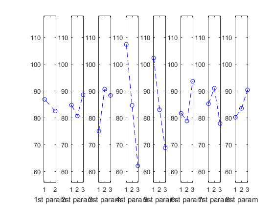
Factor Effect Chart
The factor effect diagram is a graph expressing the effect of each factor, with the horizontal axis representing the level of the factor and the vertical axis representing the S / N ratio and the characteristic value. From this graph, find the condition with high S / N ratio and select the one with better characteristics.
factoreffectchart is my helper function.
S/N ratio
According to this chart, the S/N ratio is very good at both the 1st level of the 4th and 5th parameters (or variables).
The 4th variable is the x radius and the 5th variables is the y radius.
d = orthogonalarray('L18');
Osn = factoreffectchart(d,results.sn) % S/N
Osn =
       86.873       82.546          NaN
       84.781       80.741       88.608
        75.07       90.698       88.362
       107.35       84.679       62.103
       102.29       83.019       68.818
        81.69       78.818       93.621
       85.258        91.02       77.851
       80.213       83.509       90.407
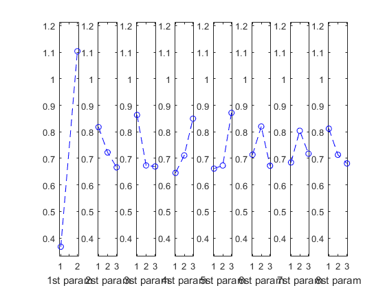
Output
To minimize the strain, the 1st level of the 1st variable is good.
The 1st variable is material.
We succeed at reducing the parameters from 7 variables to 4.
O = factoreffectchart(d,results.output) % Output
O =
      0.36726       1.1035          NaN
      0.81783      0.72215      0.66618
      0.86336      0.67327      0.66952
      0.64534      0.71116      0.84967
      0.66149      0.67315      0.87153
      0.71387      0.82003      0.67226
      0.68465      0.80391       0.7176
      0.81182      0.71343       0.6809
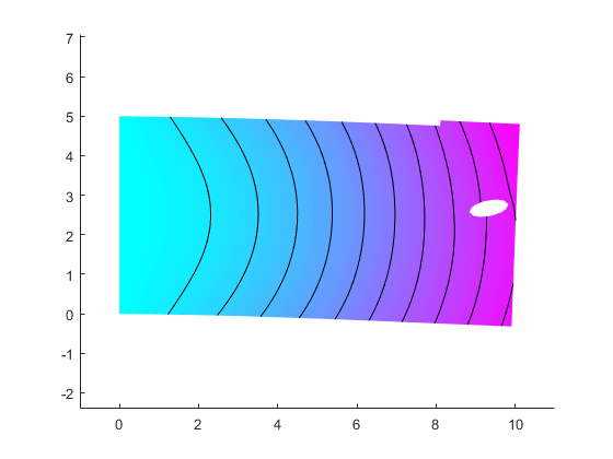
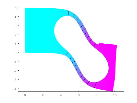
Optimization using patternsearch solver
We will optimize 4 parameters using the patternsearch solver.
First of all, we are going to optimize the location of the hole that minimizes strain.
The objective function is the code from 192 to 197 lines in "pdesample.m".
dbtype pdesample 193:197

close all
193   function out = myobjfun(in)
194
195   out = pdesample_input([1 in(1) in(2) 0.5 0.2 in(3) in(4)]);
196
197   end
opt = optimoptions('patternsearch');
opt.MeshTolerance = 0.001;
opt.FunctionTolerance = 0.00001;
opt.MaxIterations = 500;
opt.TimeLimit = 10*60;
opt.UseParallel = true;
opt.Display = 'iter';
[x,obj] = patternsearch(lh{3}, [7,3,0.2,0],[],[],[],[],[2.0,0.3,0.1,-pi/4],[9.5,4.5,0.3,pi/4],lh{5},opt)
                                      Max
  Iter   Func-count       f(x)      Constraint   MeshSize      Method
    0         1     0.338279            0            1
    1         6      0.33769            0     0.009772   Update multipliers
    2       329     0.334631            0     0.000955   Update multipliers
Optimization terminated: mesh size less than options.MeshTolerance
 and constraint violation is less than options.ConstraintTolerance.
x =
       9.3125       2.9688      0.14141         0.25
obj =
      0.33463
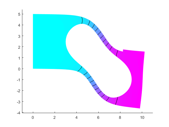
Optimization using ga solver
We will also optimize 4 parameters using the ga> solver.
gaoptions = gaoptimset(@ga);
gaoptions.CrossoverFcn = @crossoverintermediate;
gaoptions.MutationFcn = @mutationadaptfeasible;
gaoptions.CrossoverFraction = 0.5;
gaoptions.TolFun = 0.00001;
gaoptions.PopulationSize = 20; % population size

gaoptions.InitialPopulation = [7,3,0.2,0]; % initial population
gaoptions.Generations = 500; %
gaoptions.TimeLimit = 10*60;
gaoptions.UseParallel = true;
gaoptions.Display = 'iter';

[x,fval]  = ga(lh{3},4,[],[],[],[],[2.0,0.3,0.1,-pi/4],[9.5,4.5,0.3,pi/4],lh{5},gaoptions)
                              Best       Max        Stall
Generation  Func-count        f(x)     Constraint  Generations
    1           1078       0.33505            0      0
    2           1598      0.334569    0.0008296      0
Optimization terminated: average change in the fitness value less than options.FunctionTolerance
 and constraint violation is less than options.ConstraintTolerance.
x =
       9.3345       3.1148      0.19511      0.36912
fval =
      0.33457
The values of the output by both the patternsearch and ga solvers are reduced from the inital conditions. Both results give especially similiar results for the x,y positions. We conclude that both results are good. However, the area of hole is the smallest possible because of considering the S/N ratio. In order to lighten the weight, we will enlarge the area of hole.
Multi-objective optimization using the gamultiobj solver
We would like to optimize both the size and location of the hole in order to minmize the strain and lighten the weight.
In the previous case, radius x and y are the minimum values. In order to increase the size of the hole, we will use a multi-objective optimization gamultiobj solver.
The relationship between the value of strain and the area of hole is inverse proportional and there is a trade-off.
The objective function is the code from 200 to 205 lines in "pdesample.m".
dbtype pdesample 200:205
200   function out = myobjfun2(in)
201
202   out(1) = pdesample_input([1 in 0.2 0*pi/12]);
203   out(2) = -pi*in(3)*in(4);
204
205   end
mulgaoptions = gaoptimset(@gamultiobj);
mulgaoptions.CrossoverFraction = 0.5;
mulgaoptions.TolFun = 0.001;
mulgaoptions.PopulationSize = 100;
mulgaoptions.Generations = 3000;
mulgaoptions.InitialPopulation = [7 2.5 0.5 0.5];
mulgaoptions.UseParallel = false;
mulgaoptions.TimeLimit = 20*60;
[x,fval,exitflag,output]  = gamultiobj(lh{4},4,[1 0 1 0;0 1 0 1;-1 0 1 0; 0 -1 0 1],[9.9;4.9;-0.2;-0.2],[],[],[2.0,0.3,0.2,0.2],[9.6,4.5,3,2.6],mulgaoptions);
Optimization terminated: time limit exceeded.
Here is the biggest hole.
lh{4}(x(1,:))
ans =
      0.33632     -0.62854
In this next plot, we show the pareto frontier which is popular for design engineering. There you can see the trade-off between area and strain for making design decisions.
scatter(fval(:,1),50.4 + fval(:,2),'m')
set(gca,'FontSize',16,'FontName','Meiryo UI')
xlabel('strain');ylabel('area');title('pareto frontier')
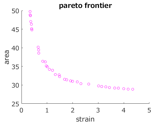
Pareto frontier results.
T1 = array2table([fval(:,1) 50.4+fval(:,2) x],'VariableNames',{'Strain','Area','x','y','rx','ry'})
T1 =
  35×6 table
    Strain      Area       x          y         rx         ry
    _______    ______    ______    _______    _______    _______
    0.33632    49.771    8.4674    0.83566    0.54447    0.36746
     2.9137    29.829    6.1874     2.4294     2.9804      2.197
     0.8458    36.385    6.1587     2.0938     2.7957     1.5957
     3.9636    29.123    6.1812      2.593     2.9923     2.2634
      1.553    32.151     5.883     2.3126     2.9526     1.9674
    0.83451    37.023    6.7695     2.1714     2.4951     1.7065
    0.42155    44.452     7.107     2.1224     1.3364     1.4167
     1.2357    33.732    6.0206     2.5458      2.879     1.8429
    0.93663    35.477    6.1315     2.3105     2.9743     1.5971
    0.75125    37.875    6.7413     2.0409     2.5471     1.5653
     1.0758     34.69     6.385     2.4479     2.8222     1.7719
      3.077    29.714    6.1778     2.4877     2.9777     2.2113
     2.8688    29.875     6.022     2.4611     2.9817     2.1911
    0.39498    45.353    7.3136     1.8261     1.4593     1.1008
     1.1526    34.152    6.2626     2.1237     2.9141     1.7747
    0.35257     47.25    8.2497     1.2095     1.0588    0.94702
     3.4396    29.299    6.3585     2.4648          3     2.2389
     1.4782    32.434    6.1279     2.4721     2.9814     1.9181
     2.1484    30.683    5.9299     2.4064     2.9995     2.0924
    0.50403    41.862    7.0168     2.0862     1.8298     1.4853
     2.3041    30.529    5.9573     2.4324     2.9834     2.1201
     1.6972    31.718    5.9601     2.4295     2.9809      1.995
     3.2141    29.467    6.1923     2.4677          3      2.221
    0.34045    48.795    8.1318     1.0284     0.8714    0.58627
     1.0626    35.115    6.6304     2.3413     2.6315     1.8489
     1.3309    33.168     6.023     2.5945     2.9801     1.8405
    0.38738    45.534    7.4165     1.5702     1.5472     1.0012
     1.4303    32.719    5.9897      2.279     2.8842     1.9514
    0.55291    40.816    5.8008     1.8469      2.672     1.1418
     1.8278    31.425    5.9551      2.491     2.9899     2.0201
     0.3506    48.091    8.7273     1.5772    0.62704      1.172
     1.9699     31.13    6.0712     2.4664       2.98     2.0583
     3.7843    29.133    6.0624     2.4919     2.9961     2.2595
     2.7137    30.065     6.191     2.4831     2.9761     2.1749
     3.6181    29.252    5.7451     2.5008     2.9962     2.2467
Conclusion
We showed how to use FEM tools and Optimization Toolbox to perform structural design. What can you shape with these tools? Let us know your thoughts here.


댓글
댓글을 남기려면 링크 를 클릭하여 MathWorks 계정에 로그인하거나 계정을 새로 만드십시오.