Loren’s Excellent Adventure: Maps, Graphs, and Polygons
R2017b was released recently. Today's guest blogger, Matt Tearle, discovered a fun application of one of the many new features - solving a map-based puzzle.
Contents
A traveling MathWorker problem
"Car Talk" recently featured a brain teaser submitted by a former MathWorker. The short, slightly modified version is: Loren has to drive from Delaware to every state in the contiguous US, visiting each state exactly once; Loren's boss - let's call him Jack - offers to meet her in the last state, which turns out to be his birthplace; but how can Jack know what the last state will be, without waiting to hear Loren's itinerary?
I'm about to give away the answer, so if you want to figure it out yourself, do so now. It's OK, I'll wait.
Done? Great. Hopefully you realized that there's one and only one state that borders only one other state. That state has to be the beginning or end of any path. (You can't visit any state more than once so once you enter from the single neighboring state, you're stuck.) The beginning is Delaware (which borders several other states), so this unique "degree-one" state must be the end of Loren's epic journey.
Enter MATLAB
As usual for me, the really interesting aspect of this problem is: can I solve it in MATLAB? This is a classic "traveling salesman" problem, so the graph capabilities recently added to MATLAB should be of use. But the first problem is how to build the graph that represents the connections between the states. It turns out that another new feature will help.
A new variable type for representing 2-D polygons was introduced in R2017b. The polyshape function takes vectors representing x and y coordinates and returns a polygon with those points as its vertices. It so happens that Mapping Toolbox comes with a data file containing the latitudes and longitudes of the borders of the US states - just what I need. With the shaperead function I can import this data in the form of a structure array, with fields for the name of the state and the latitude/longitude of the border:
states = shaperead('usastatehi.shp');
% Remove Alaska & Hawaii, and Washington DC
states([2,11,51]) = [];
For a single state, it's straightforward to extract the arrays in the X (longitude) and Y (latitude) fields and use these as the inputs to polyshape:
x = states(1).X;
y = states(1).Y;
p = polyshape(x,y)
p =
  polyshape with properties:

      Vertices: [518×2 double]
    NumRegions: 2
      NumHoles: 0
Now that the state is represented as a polygon, I can use the functions that can work with polygon, such as plotting:
plot(p)

But to really get the benefit of working with polygons, I'd like to get an array of them, where each element is a polygon representing one state. I could extract the x and y components for each state in a loop, but any time I see myself about to apply an operation to each element of an array, I think "time for arrayfun!".
struct2poly = @(s) polyshape(s.X,s.Y); % define my struct -> polyshape operation
p = arrayfun(struct2poly,states) % apply to all elements of the struct STATES
p =
  48×1 polyshape array with properties:

    Vertices
    NumRegions
    NumHoles
Because this is MATLAB, functions like plot should work on arrays of polygons, just as well as scalar polygons, right?
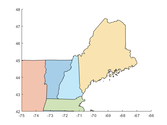
plot(p)

Isn't that nice? Each polygon is plotted as its own shaded shape. If we zoom in, we can see the solution to the puzzle.
axis([-75 -66 42 48])

Problem: who is my neighbor?
By eye we can see how states share borders, but how can we get MATLAB to determine this in an automated way? Let's start with the simplest problem: given two states (polygons), can we determine if they share a border or not?
me = p(17);
ma = p(19);
nh = p(27);
subplot(1,2,1)
plot([ma nh])
title('Shared border')
subplot(1,2,2)
plot([ma me])
title('No shared border')

The polygons have a Vertices property that contains the border locations. So a simplistic approach would be to see if the two polygons have any vertices in common. However, this has a lot of potential problems. Firstly, two shapes can share a boundary without sharing vertices:
a = polyshape([0 1 1 0],[0 0 3 3]);
b = polyshape([1 2 2 1],[1 1 2 2]);
subplot(1,1,1)
plot([a b])
intersect(a.Vertices,b.Vertices,'rows')
ans =
  0×2 empty double matrix

Secondly, even if the survey points all align, there's always the potential for floating-point precision issues: how is 31°41'59" represented?
lat1 = 31.699722222222222
lat2 = 31 + 41/60 + 59/3600
lat1 == lat2
lat1 - lat2
lat1 =
         31.7
lat2 =
         31.7
ans =
  logical
   0
ans =
  -3.5527e-15
So a better idea might be to think about it geometrically. Two areas in the plane share a border if their intersection is a line or curve. And the new polygons in MATLAB have an intersect functionality! However, unfortunately, from a programming perspective, the intersection of two polygons is another polygon. And a polygon with zero area (which you get when the intersection is a line) is empty, so there's no obvious way to distinguish between states that share a boundary or not.
intersect(ma,nh)
intersect(ma,me)
ans =
  polyshape with properties:

      Vertices: [0×2 double]
    NumRegions: 0
      NumHoles: 0
ans =
  polyshape with properties:

      Vertices: [0×2 double]
    NumRegions: 0
      NumHoles: 0
Furthermore, this approach would still have been vulnerable to the finite precision problem.
Solution: the fat of the land
The new MATLAB polygons have a polybuffer function that gives you a way to "fatten up" a polygon by pushing the border out a given amount. Here's Massachusetts with a 0.1-degree (approx. 7-mile) border:
mafat = polybuffer(ma,0.1);
plot([ma mafat])

This gives a fairly simple, but robust, way to determine whether states are neighbors: put a small buffer around both and then see if there's any overlap.
pfat = polybuffer(p,1e-4); % add ~35 feet around every state
me = pfat(17);
ma = pfat(19);
nh = pfat(27);
intersect(ma,nh)
intersect(ma,me)
ans =
  polyshape with properties:

      Vertices: [541×2 double]
    NumRegions: 1
      NumHoles: 0
ans =
  polyshape with properties:

      Vertices: [0×2 double]
    NumRegions: 0
      NumHoles: 0
As you'd expect for a data type that represents polygons, there's an area function that does exactly what its name suggests:
area(intersect(ma,nh))
area(intersect(ma,me))
ans =
   0.00035462
ans =
     0
So determining whether the padded states overlap should be simple: does the intersection have nonzero area? But the programmer in me was a bit worried: should I use a function, like area, that will come with some overhead? Would it be more efficient to directly query the properties of the polygon that results from the intersection?
However, there's another slight wrinkle that needs to be considered before worrying about implementation details. The "Four Corners" area of the American Southwest is the one place where four states touch - Colorado, New Mexico, Arizona, and Utah. Does Colorado border Arizona? Does Utah border New Mexico? We can let philosophers and mathematicians argue over that. But unless an infinitely thin Loren is driving an infinitely thin car, the answer, for our purposes, is no. There's no way in reality to drive from Colorado to Arizona without going through Utah or New Mexico.
plot(pfat,'LineStyle','none')
axis([-109.055 -109.035 36.99 37.01])

But if we look at the intersection between the "fattened" states, there will be a small overlap between Colorado and Arizona. Note that it will be very small - only slightly bigger than my apartment in graduate school, which should probably be considered a quantum amount of geographic area. Any real border between states will be at least an order of magnitude larger than this. So now we have a simple and robust way to determine whether or not states share a border:
- Add a small border to all states
- Compute the area of the intersection of states
- States share a border if that intersection is greater than a threshold
area(intersect(ma,nh)) > 1e-6
area(intersect(ma,me)) > 1e-6
ans =
  logical
   1
ans =
  logical
   0
Now I just need to apply that to every pair of states. I could probably try to get fancy with arrayfun, but this is a case where the simple for-loop approach might be a better idea. In fact, loops can help me avoid redundant calculations. If State A borders State B, then State B borders State A and I don't have to check that.
border = zeros(48);
for k = 1:48
    for j = (k+1):48 % Only need j for ks we haven't checked yet
        border(j,k) = area(intersect(pfat(j),pfat(k))) > 1e-6;
    end
end
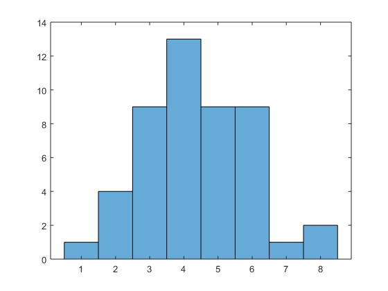
The result of this is a lower-triangular matrix of connections. Now I can build a graph from the connectivity matrix and solve the problem. One of the neat graph functions is degree, which gives the number of connections to each node.
G = graph(border,'lower');
histogram(degree(G))

So there's one degree-one node in the graph. That's the one we want. But which state does that correspond to? The names are stored in the Name field of the original structure array. I'll extract them into a cell array by using one of my favorite MATLAB tricks. When indexing produces multiple results (not just an array with multiple elements), those results come back in the form of a comma-separated list. That is, if s is a structure array (for example), s.Thing is equivalent to s(1).Thing, s(2).Thing, ..., s(end).Thing. What's great about having a comma-separated list is that that's the form MATLAB uses for concatenating elements into an array (i.e., [a,b,c] or {a,b,c}) and for passing inputs into a function (i.e., myfun(a,b,c)). Hence, I can extract all the Name field elements of the structure array states and concatenate them into a cell array with one simple line of MATLAB:
stnames = {states.Name};
And now, finally, I can find out which state borders only one other state:
stnames{degree(G) == 1}
ans =
    'Maine'
Visualizing the results
Having the state names, I can go a little further and visualize both the map and the connectivity graph. To start, it's possible to name the nodes in a graph:
G = graph(border,stnames,'lower');
This is useful when you visualize a graph because the nodes are automatically labeled:
plot(G)

But this graph doesn't show the states in a physical layout. It's also possible to specify the locations of the nodes when plotting a graph, but for that I need a point in each state to use as the node location. Right in the middle of the state would be good... Guess what? There's a polygon function for that: centroid.
[x,y] = centroid(p);
plot(G,'XData',x,'YData',y)

That's looking pretty good. It would be nice to add the map for reference.
plot(p)
hold on
plot(G,'XData',x,'YData',y)
hold off

Nice! Something cool to notice about that code: two uses of plot, both of which were on "exotic", non-numeric data types (one polygon array and one graph). This is something that our management team work hard on - making sure functionality is consistent, so that, for example, plot works naturally on different kinds of data. It's a feature of MATLAB I greatly appreciate. It means that I, as a MATLAB user, don't have to expend brain energy on which plotting function, or even which variant of plot, I have to use. I can just use plot and get on with what I'm actually trying to do.
Where to next?
I solved the brain teaser, and even went a bit further to make a nice visualization of the states and their connections. But there's one thing about my visualization that's still bugging me: the states are colored with seven unique colors in the order that the states appear in the polygon array (which happens to be alphabetical by name). This means that neighboring states are sometimes given the same color. For example, note that Nebraska and the Dakotas are elments 25, 32, and 39, which means they all end up the same color. I happen to recall that there's a mathematical theorem that says that any map can be colored with only four unique colors, such that no neighboring regions have the same color.
To me, that sounds like a second interesting task for polygons and graphs,... but a story for another time. In the meantime, let us know in the comments if you can think of somewhere in your work where the new polyshape type might be useful.


Comments
To leave a comment, please click here to sign in to your MathWorks Account or create a new one.