What’s New in Simulink R2025a!

著者 Guy Rouleau, May 16, 2025

283 ビュー (過去 30 日間) | 0 いいね | 2 コメント

For a first post about R2025a, I decided to highlight 3 enhancements that will help speed up your Simulink workflows... and since it helped me writing this post, a quick mention of the new MATLAB Copilot

Fast Restart for Rapid Accelerator

A few years ago, I published this post: Getting the most out of Rapid Accelerator mode – Version R2023b » Guy on Simulink - MATLAB & Simulink. In R2025a, we made this workflow simpler and more efficient.

It's as simple as specifying UseFastRestart='on' when calling sim for a model in Rapid Accelerator mode. The benefit is that subsequent simulations will restart much faster.

Let's take this simple model:

mdl = 'RapidAccelFastRestart';

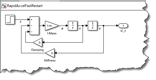
I will run 10 simulations in Rapid Accelerator mode with 10 different values for k.

N = 10;

kValues = 10*(1:10);

Let's first build the Rapid Accelerator target:

Simulink.BlockDiagram.buildRapidAcceleratorTarget(mdl);

### Searching for referenced models in model 'RapidAccelFastRestart'.
### Total of 1 models to build.

As a reference, I will run the simulation "old style" using RapidAcceleratorUpToDateCheck=Off:

in = repmat(Simulink.SimulationInput(mdl),N,1);

for i = 1:N

    in(i) = in(i).setVariable('k', kValues(i));

    in(i) = in(i).setModelParameter('SimulationMode','Rapid');

    in(i) = in(i).setModelParameter('RapidAcceleratorUpToDateCheck','off');

end

outOld = sim(in,'ShowProgress','Off');

With the Fast Restart option, the code we recommend in R2025a is:

in = repmat(Simulink.SimulationInput(mdl),N,1);

for i = 1:N

    in(i) = in(i).setVariable('k', kValues(i));

    in(i) = in(i).setModelParameter('SimulationMode','Rapid');

end

outNew = sim(in,'ShowProgress','Off','UseFastRestart','on');

figure

hold on

arrayfun(@(x) outNew(x).yout{1}.Values.plot,1:N)

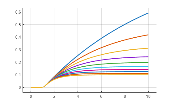
(yes... I know... I started to use arrayfun on arrays of SimulationOuput objects recently and I am probably having too much fun with it)

Let's sum the time for those two runs:

sum(arrayfun(@(x) outOld(x).SimulationMetadata.TimingInfo.TotalElapsedWallTime,1:N))

ans = 27.6707

sum(arrayfun(@(x) outNew(x).SimulationMetadata.TimingInfo.TotalElapsedWallTime,1:N))

ans = 5.0618

This large difference (30 seconds vs 6 seconds) is due to the fact that, traditionally, each simulation in Rapid Accelerator mode needs to launch a separate executable, which takes 1-2 seconds. In R2025a, we can keep the Rapid Accelerator executable running and restart the simulation. This makes this enhancement especially relevant for cases where you need to run tons of simulations for which the execution time is small.

Variable-Step Local Solver

Model Reference Local Solver has seen incremental improvements since its initial release in R2022a. In R2025a, we are making a major step forward with support for variable-step local solver.

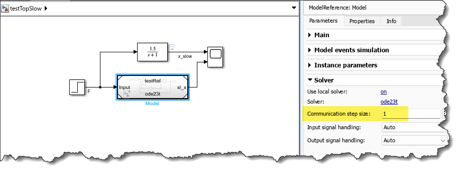
To illustrate the benefit, let's take this example where a top model has continuous states capturing a slow dynamic, and it references a second model, also with continuous states, but with a faster dynamic. 

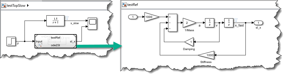
Without local solver, Simulink needs to solve all the continuous states with the same solver, taking the same time steps. Let's take this example:

mdl = 'testTopSlow';

in = Simulink.SimulationInput(mdl);

mdlRef = 'testRef';

load_system(mdlRef);

set_param(mdlRef,'UseModelRefSolver','off');

out = sim(in); %#ok<NASGU>

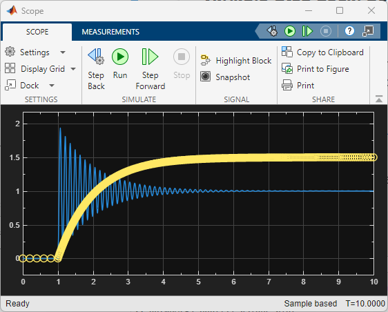
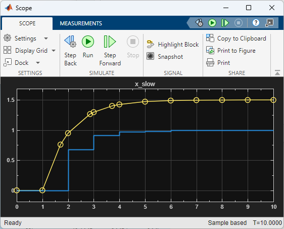
Looking at the markers in this Scope, it's a lot of small unnecessary small steps to solve the slow dynamic of the top model.

In R2025a, it is possible to enable local solver for the referenced model and solve it with a stiff solver like ode23t, while the top model can take large steps.

set_param(mdlRef,'UseModelRefSolver','on')

out = sim(in);

To confirm that the referenced model has really been solved at the faster rate, we can look at the signal logged inside it and confirm that it contains a lot more points than the one outside:

length(out.logsout.get("x_slow").Values.data)

ans = 16

length(out.logsout.get("x_fast").Values.data)

ans = 708

As illustrated by this example, this feature needs to be used with caution, because the top model will only exchange data with the referenced model at the rate specified by the communication step size specified in the model block:

In addition to variable-step solver, local solver also removed multiple limitations and now supports: Zero-crossing detection, instance parameter, operating point, and fast restart support for fixed-step and variable-step local solvers.

Flexible Operating Point

Are you familiar with operating points and Speed Up Simulation Workflows by Using Model Operating Points - MATLAB & Simulink?

For many releases, this feature has allowed you to simulate a model up to a certain stop time, save an operating point and then restart multiple simulations from this operating point. Here is an example:

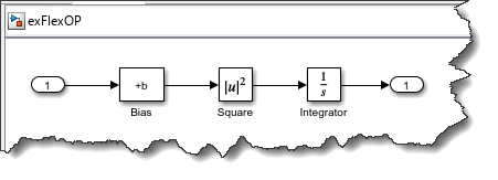
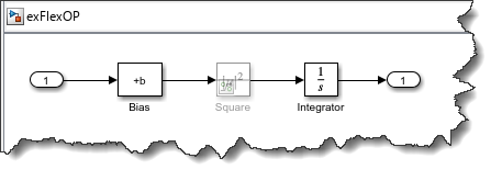
mdl = 'exFlexOP';

open_system(mdl);

Simulate the model once for 10 seconds

in = Simulink.SimulationInput(mdl);

in = in.setModelParameter('SaveFinalState', 'on');

in = in.setModelParameter('SaveOperatingPoint', 'on');

in = in.setModelParameter('FinalStateName', 'myOp');

in = in.setModelParameter('StopTime','10');

out1 = sim(in);

Let's use the operating point and simulate for 10 to 12 seconds, with multiple values for b

in = repmat(Simulink.SimulationInput(mdl),5,1);

for i = 1:length(in)

    in(i) = in(i).setModelParameter('LoadInitialState','on');

    in(i) = in(i).setModelParameter('InitialState','out1.myOp');

    in(i) = in(i).setModelParameter('StopTime','12');

    in(i) = in(i).setVariable('b',-i);

end

out2 = sim(in,'ShowProgress','Off','UseFastRestart','on');

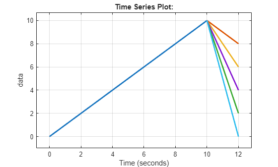
Let's plot the results:

figure

plot(out1.yout{1}.Values)

hold on

arrayfun(@(x) out2(x).yout{1}.Values.plot,1:length(in));

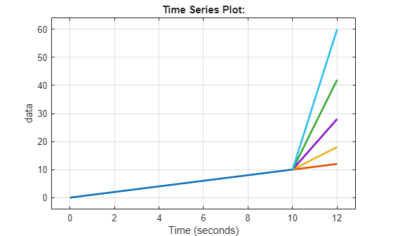
In this case, we only tuned the value of a parameter, which was supported in previous releases. Next, let's look at what the R2025b enhancement enables.

Modifying the model and restarting

For many reasons, you might need to modify the model and still want to restore simulations from the operating point. For this example, let's comment through the Square block and re-run the simulations, which would have previously errored out.

For that, you need to explicitly set the diagnostic Operating point contents checksum mismatch to warning or none.

in = repmat(Simulink.SimulationInput(mdl),5,1);

for i = 1:length(in)

    in(i) = in(i).setModelParameter('OperatingPointContentsChecksumMismatchMsg','none');

    in(i) = in(i).setBlockParameter('exFlexOP/Square','Commented','through');

    in(i) = in(i).setModelParameter('LoadInitialState','on');

    in(i) = in(i).setModelParameter('InitialState','out1.myOp');

    in(i) = in(i).setModelParameter('StopTime','12');

    in(i) = in(i).setVariable('b',-i);

end

out2 = sim(in,'ShowProgress','Off');

Let's plot the results:

figure

plot(out1.yout{1}.Values)

hold on

arrayfun(@(x) out2(x).yout{1}.Values.plot,1:length(in));

MATLAB Copilot

This is not a Simulink-specific feature, but since it helped me write this blog post, I thought I should highlight it. MATLAB now has a Copilot!

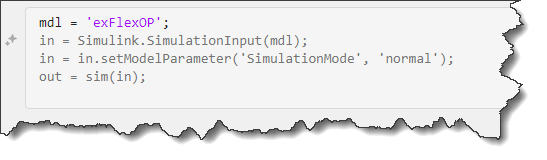
While writing the above section, I only typed 

mdl = 'exFlexOP';

and Copilot offered this, which is quite close to what I needed:

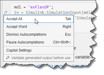
All I had to do is hit Tab or click on the Copilot icon and hit Accept All:

As I continued coding, I added a comment saying I wanted to simulate for 10 seconds, and it immediately offered me this line to set the stop time to 10 seconds:

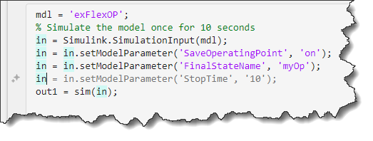
I think I will like that feature.

Now it's your turn

Give a look at the Simulink release notes and let us know in the comments below what's your favorite feature and which ones you would like to hear about in more details on this blog.