
Colormap Test Image
Today I want to tell you how and why I made these images:

After the MATLAB R2014b release, I wrote several blog posts (Part 1, Part 2, Part 3, and Part 4) about the new default colormap, parula, that was introduced in that release.
Sometime later, I came across some material by Peter Kovesi about designing perceptually uniform colormaps (or colourmaps, as Peter writes it).
I was particularly intrigued by a test image that Peter designed for the purpose of visually evaluating the perceptual characteristics of a colormap.
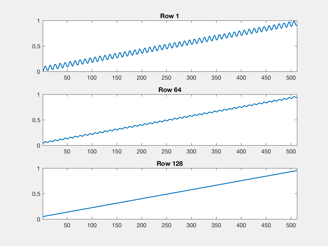
The image is constructed by superimposing a sinusoid on a linear ramp, with the amplitude of the sinusoid getting smaller as you move away from the top row. Here are three cross-sections of the image: row 1, row 64, and row 128.
url = 'http://peterkovesi.com/projects/colourmaps/cm_MATLAB_gray256.png';
I = im2double(imread(url));

subplot(3,1,1)
plot(I(1,:))
axis([1 512 0 1])
title('Row 1')

subplot(3,1,2)
plot(I(64,:))
axis([1 512 0 1])
title('Row 64')

subplot(3,1,3)
plot(I(128,:))
axis([1 512 0 1])
title('Row 128')
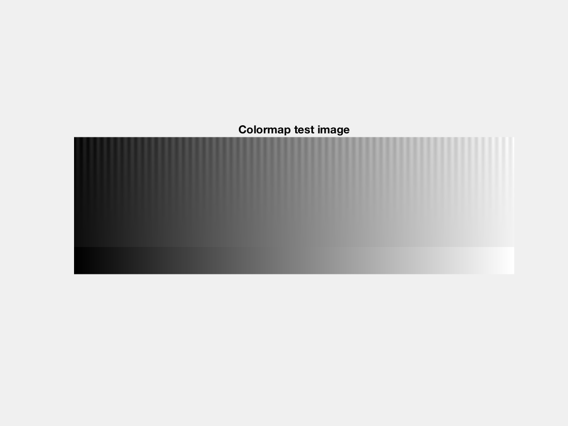
Here is the basic code for making this test image. I'm going to vary Kovesi's image slightly. I'll add an extra half-cycle of the sinusoid so that it reaches a peak at the right side of the image, and I'll add a full-range linear ramp section at the bottom. (If you look closely at the cross-section curves above, you'll see that the linear ramp goes from 5% to 95% of the range.)
First, compute the ramp.
num_cycles = 64.5;
pixels_per_cycle = 8;
A = 0.05;
width = pixels_per_cycle * num_cycles + 1;
height = round((width - 1) / 4);
ramp = linspace(A, 1-A, width);
Next, compute the sinusoid.
k = 0:(width-1);
x = -A*cos((2*pi/pixels_per_cycle) * k);
Now, vary the amplitude of the sinusoid with the square of the distance from the bottom of the image.
q = 0:(height-1);
y = ((height - q) / (height - 1)).^2;
I1 = (y') .* x;
Superimpose the sinusoid on the ramp.
I = I1 + ramp;
Finally, add a full-range linear ramp section to the bottom of the image.
I = [I ; repmat(linspace(0,1,width), round(height/4), 1)];

clf
imshow(I)
title('Colormap test image')
Last week, I posted Colormap Test Image to the File Exchange. It contains the function colormapTestImage, which does all this for you.
I = colormapTestImage;
The function has another syntax, too. If you pass it the name of a colormap, it will display the test image using that colormap. For example, here is the test image with the old MATLAB default colormap, jet.
colormapTestImage('jet')
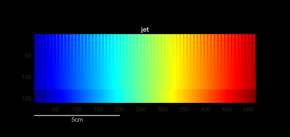
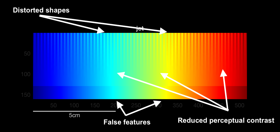
This test image illustrates why we replaced jet as the default MATLAB colormap. I have annotated the image below to show some of the issues.
Now compare with the new default colormap, parula.
colormapTestImage('parula')

I think that illustrates what we were trying to achieve with parula: perceptual fidelity to the data.
Since I'm talking about parula, I'll finish by mentioning that we need some very subtle tweaks to parula in the R2017b release. So you can compare, I'll show you the original version that shipped with R2014b.
colormapTestImage('parula_original')
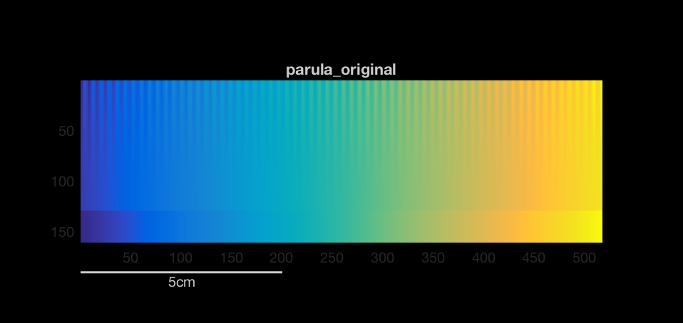
Readers, can you tell what is different? Let us know in the comments.
- Category:
- Colormap


Comments
To leave a comment, please click here to sign in to your MathWorks Account or create a new one.