
It's reached that time for me. I will be retiring from MathWorks at the end of March 2022. It's been 35 years of tremendous growth for MathWorks, and for me. When I started this blog, the original... read more >>

Note
Loren on the Art of MATLAB has been archived and will not be updated.
It's reached that time for me. I will be retiring from MathWorks at the end of March 2022. It's been 35 years of tremendous growth for MathWorks, and for me. When I started this blog, the original... read more >>


Today's guest blogger is Matt Tearle, who works on the team that creates our online training content, such as our various Onramp courses to get you started on MATLAB, Simulink, and applications.... read more >>

Today's guest blogger is Adam Filion, a Senior Data Scientist at MathWorks. Adam has worked on many areas of data science at MathWorks, including helping customers understand and implement data... read more >>

In the early 1990s, to avoid eval and all of its quirks (if you don't know about this, DON'T look it up - it's totally discouraged), we recommended using feval for evaluating functions that might... read more >>
Benefits of Refactoring CodeI have seen a lot of code in my life, including code from many different people written for many different purposes, and in many different "styles". These styles range... read more >>

Seventeen? Why 17? Well, as a high school student, I attended HCSSIM, a summer program for students interested in math. There we learned all kinds of math you don't typically learn about until... read more >>
Today I want to introduce you to Jake Mitchell, a MATLAB user that I knew of and someone recently reminded me of again. Jake is a mechanical engineering major who is interested in data science. He... read more >>
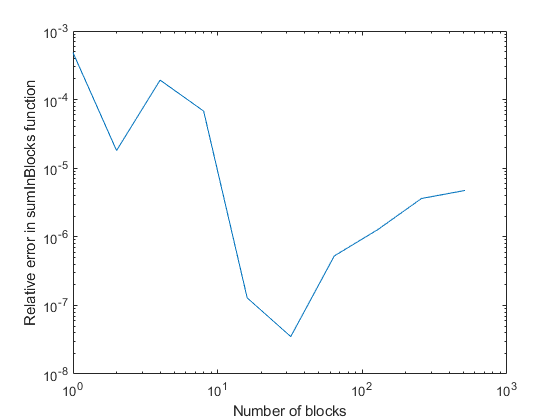
Today's guest blogger is Christine Tobler, who's a developer at MathWorks working on core numeric functions.Hi everyone! I'd like to tell you a story about round-off error, the algorithm used in sum,... read more >>
Today's guest blogger is Alan Weiss, who writes documentation for Optimization Toolbox™ and other mathematical toolboxes.Table of ContentsCone Programming Discrete Dynamics With Cone... read more >>

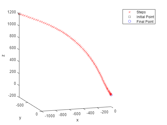
Have you ever needed to solve an optimization problem where there were local minima? What strategy do you use to solve it, trying to find the "best" answer? Today I'm going to talk about a simple... read more >>
These postings are the author's and don't necessarily represent the opinions of MathWorks.