Have you ever needed to solve an optimization problem where there were local minima? What strategy do you use to solve it, trying to find the "best" answer? Today I'm going to talk about a simple strategy, readily available in the Global Optimization Toolbox. Solve a Simple Problem
Or at least let's try. I have some data and I want to fit a particular form of a curve to it. First let's look at the pharmacokinetic data. Here's the reference: Parameter estimation in nonlinear algebraic models via global optimization. Computers & Chemical Engineering, Volume 22, Supplement 1, 15 March 1998, Pages S213-S220 William R. Esposito, Christodoulos A. Floudas.
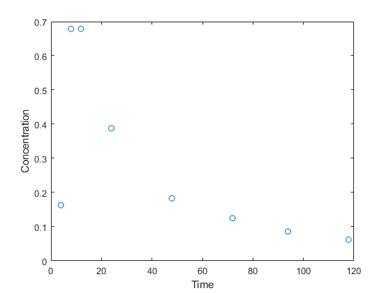
The data are time vs. concentration
t = [ 3.92, 7.93, 11.89, 23.90, 47.87, 71.91, 93.85, 117.84 ]
3.9200 7.9300 11.8900 23.9000 47.8700 71.9100 93.8500 117.8400
c = [0.163, 0.679, 0.679, 0.388, 0.183, 0.125, 0.086, 0.0624 ]
0.1630 0.6790 0.6790 0.3880 0.1830 0.1250 0.0860 0.0624
I like to see the data, in part to be sure I have no entry mistakes, and in part to get a feel for the overall system. In fact, let's visualize the data.
3 Compartment Model
As in the reference, we fit a 3 compartment model, sum of 3 decaying exponentials.
and we can express that model as an anonymous function of t (time) and the model parameters [b(1) b(2) ... b(6)]. model = @(b,t) b(1)*exp(-b(4)*t) + b(2)*exp(-b(5)*t) + b(3)*exp(-b(6)*t)
model =
@(b,t)b(1)*exp(-b(4)*t)+b(2)*exp(-b(5)*t)+b(3)*exp(-b(6)*t)
Define Optimization Problem
We next define the optimization problem to solve using the problem-based formulation. This allows us to choose the solver we want, supply the data, and naturally express constraints and options. problem = createOptimProblem('lsqcurvefit', ...
'xdata', t, 'ydata', c, ...
'lb', [-10 -10 -10 0 0 0 ],...
'ub', [ 10 10 10 0.5 0.5 0.5], ...
'options',optimoptions('lsqcurvefit',...
'OutputFcn', @curvefittingPlotIterates,...
'Display','none'))
problem =
objective: @(b,t)b(1)*exp(-b(4)*t)+b(2)*exp(-b(5)*t)+b(3)*exp(-b(6)*t)
x0: [1 1 1 1 1 1]
xdata: [3.9200 7.9300 11.8900 23.9000 47.8700 71.9100 93.8500 117.8400]
ydata: [0.1630 0.6790 0.6790 0.3880 0.1830 0.1250 0.0860 0.0624]
lb: [-10 -10 -10 0 0 0]
ub: [10 10 10 0.5000 0.5000 0.5000]
solver: 'lsqcurvefit'
options: [1×1 optim.options.Lsqcurvefit]
Solve the Problem
First solve the problem directly once.
b = lsqcurvefit(problem)
0.1842 0.1836 0.1841 0.0172 0.0171 0.0171
You'll notice that the model does not do a stellar job fitting the data or even following the shape of the data.
MultiStart
Let's see if we can do better by starting at a bunch of different points.
[~,fval,exitflag,output,solutions] = run(ms, problem, 50)
Run Local Local Local Local First-order
Index exitflag f(x) # iter F-count optimality
1 3 0.222 8 63 0.0006396
2 3 0.000154 21 154 0.001864
3 3 0.009442 44 315 0.01989
4 3 1.462e-05 34 245 0.002586
5 3 1.454e-05 19 140 1.079e-05
6 3 1.475e-05 24 175 0.006883
7 3 0.009445 50 357 0.002266
8 3 1.495e-05 32 231 0.006853
9 3 1.466e-05 35 252 0.00478
10 3 0.00944 80 567 0.01042
11 3 1.471e-05 40 287 0.005472
12 3 1.566e-05 24 175 0.001576
13 3 0.009439 24 175 0.0005121
14 3 0.009451 41 294 0.02935
15 3 0.009493 26 189 0.004837
16 3 1.476e-05 40 287 0.006352
17 3 1.494e-05 40 287 0.008288
18 3 0.009446 62 441 0.01296
19 3 1.457e-05 22 161 0.001755
20 3 1.488e-05 53 378 0.007608
21 3 0.00944 37 266 0.006878
22 3 1.464e-05 24 175 0.003709
23 3 0.009449 43 308 0.02515
24 3 0.009447 47 336 0.007942
25 3 1.455e-05 23 168 0.001621
26 3 0.009442 32 231 0.01328
27 3 1.479e-05 40 287 0.004821
28 3 1.479e-05 18 133 0.006878
29 3 1.456e-05 72 511 0.0009721
30 3 1.455e-05 42 301 0.001122
31 3 0.009441 47 336 0.01537
32 3 0.009451 47 336 0.008942
33 3 0.0001729 14 105 0.0003276
34 3 0.009442 44 315 0.01062
35 3 0.0001751 21 154 7.71e-05
36 3 1.509e-05 26 189 0.009896
37 3 0.009458 39 280 0.02208
38 1 1.454e-05 24 175 7.815e-08
39 3 0.009441 60 427 0.0107
40 3 1.472e-05 34 245 0.002981
41 3 1.503e-05 22 161 0.00585
42 3 0.00952 15 112 0.008492
43 3 0.009439 21 154 0.000769
44 3 1.462e-05 64 455 0.0005576
45 3 0.009439 17 126 0.0001567
46 3 1.471e-05 30 217 0.001973
47 3 0.009444 38 273 0.02022
48 3 1.474e-05 24 175 0.004799
49 3 1.522e-05 42 301 0.008228
50 3 0.009445 40 287 0.02166
MultiStart completed the runs from all start points.
All 50 local solver runs converged with a positive local solver exit flag.
fval = 1.4540e-05
exitflag = 1
output =
funcCount: 12726
localSolverTotal: 50
localSolverSuccess: 50
localSolverIncomplete: 0
localSolverNoSolution: 0
message: 'MultiStart completed the runs from all start points.↵↵All 50 local solver runs converged with a positive local solver exit flag.'
solutions = 1×50 object
| | 1 | 2 | 3 | 4 | 5 | 6 | 7 | 8 | 9 | 10 | 11 | 12 | 13 | 14 | 15 | 16 | 17 | 18 | 19 | 20 | 21 | 22 | 23 | 24 | 25 | 26 | 27 | 28 | 29 | 30 |
|---|
| 1 | 1×1 GlobalOptimSolution | 1×1 GlobalOptimSolution | 1×1 GlobalOptimSolution | 1×1 GlobalOptimSolution | 1×1 GlobalOptimSolution | 1×1 GlobalOptimSolution | 1×1 GlobalOptimSolution | 1×1 GlobalOptimSolution | 1×1 GlobalOptimSolution | 1×1 GlobalOptimSolution | 1×1 GlobalOptimSolution | 1×1 GlobalOptimSolution | 1×1 GlobalOptimSolution | 1×1 GlobalOptimSolution | 1×1 GlobalOptimSolution | 1×1 GlobalOptimSolution | 1×1 GlobalOptimSolution | 1×1 GlobalOptimSolution | 1×1 GlobalOptimSolution | 1×1 GlobalOptimSolution | 1×1 GlobalOptimSolution | 1×1 GlobalOptimSolution | 1×1 GlobalOptimSolution | 1×1 GlobalOptimSolution | 1×1 GlobalOptimSolution | 1×1 GlobalOptimSolution | 1×1 GlobalOptimSolution | 1×1 GlobalOptimSolution | 1×1 GlobalOptimSolution | 1×1 GlobalOptimSolution |
|---|
Visualize the Best Solution
The 50th solution, which is what is plotted above, is not necessarily the best one. Luckily for us, MultiStart orders the solutions from best to worst. So we need only look at the first one. curvefittingPlotIterates(solutions)
You can see now that the 50th was not the best solution as the mean squared error on this final one displayed is over a factor of 10 better.
MultiStart with Parallel Computing
I will now see if we can improve the performance using all 4 of my cores as parallel workers locally.
run(ms, problem, 50);
Running the local solvers in parallel.
Run Local Local Local Local First-order
Index exitflag f(x) # iter F-count optimality
1 3 0.222 8 63 0.0006396
10 3 0.00944 80 567 0.01042
9 3 1.466e-05 35 252 0.00478
2 3 0.000154 21 154 0.001864
16 3 1.476e-05 40 287 0.006352
15 3 0.009493 26 189 0.004837
14 3 0.009451 41 294 0.02935
3 3 0.009442 44 315 0.01989
22 3 1.464e-05 24 175 0.003709
21 3 0.00944 37 266 0.006878
20 3 1.488e-05 53 378 0.007608
4 3 1.462e-05 34 245 0.002586
8 3 1.495e-05 32 231 0.006853
7 3 0.009445 50 357 0.002266
6 3 1.475e-05 24 175 0.006883
5 3 1.454e-05 19 140 1.079e-05
28 3 1.479e-05 18 133 0.006878
27 3 1.479e-05 40 287 0.004821
26 3 0.009442 32 231 0.01328
25 3 1.455e-05 23 168 0.001621
13 3 0.009439 24 175 0.0005121
12 3 1.566e-05 24 175 0.001576
11 3 1.471e-05 40 287 0.005472
34 3 0.009442 44 315 0.01062
33 3 0.0001729 14 105 0.0003276
32 3 0.009451 47 336 0.008942
19 3 1.457e-05 22 161 0.001755
18 3 0.009446 62 441 0.01296
17 3 1.494e-05 40 287 0.008288
24 3 0.009447 47 336 0.007942
23 3 0.009449 43 308 0.02515
31 3 0.009441 47 336 0.01537
30 3 1.455e-05 42 301 0.001122
29 3 1.456e-05 72 511 0.0009721
42 3 0.00952 15 112 0.008492
45 3 0.009439 17 126 0.0001567
37 3 0.009458 39 280 0.02208
36 3 1.509e-05 26 189 0.009896
35 3 0.0001751 21 154 7.71e-05
40 3 1.472e-05 34 245 0.002981
39 3 0.009441 60 427 0.0107
38 1 1.454e-05 24 175 7.815e-08
41 3 1.503e-05 22 161 0.00585
49 3 1.522e-05 42 301 0.008228
47 3 0.009444 38 273 0.02022
44 3 1.462e-05 64 455 0.0005576
43 3 0.009439 21 154 0.000769
48 3 1.474e-05 24 175 0.004799
50 3 0.009445 40 287 0.02166
46 3 1.471e-05 30 217 0.001973
MultiStart completed the runs from all start points.
All 50 local solver runs converged with a positive local solver exit flag.
Calculate Speedup
Speed up may not be evident until second run due to pool start up time. Since I started mine earlier, I get to see decent speed up.
speedup = serialTime/parallelTime
Do You Have Problems Where the Solution is Sensitive to the Starting Point?
Tell us about your exploration of the solution space to your problem. If the solution is sensitive to where you start, you might consider using MultiStart and other techniques from the Global Optimization Toolbox. Copyright 2021 The MathWorks, Inc.
Appendix
Here's the code for plotting the iterates.
dbtype curvefittingPlotIterates
1 function stop = curvefittingPlotIterates(x,optimValues,state)
2 % Output function that plots the iterates of the optimization algorithm.
3
4 % Copyright 2010 The MathWorks, Inc.
5
6 persistent x0 r;
7 if nargin == 1
8 showPlot(x(1).X,x(1).X0{:},x(1).Fval)
9 else
10 switch state
11 case 'init' % store initial point for later use
12 x0 = x;
13 case 'done'
14 if ~(optimValues.iteration == 0)
15 % After optimization, display solution in plot title
16 r = optimValues.resnorm;
17 showPlot(x,x0,r)
18 end
19 end
20 end
21 if nargout > 0
22 stop = false;
23 clear function
24 end
25 end
26
27 function showPlot(b,b0,r)
28 f = @(b,x) b(1)*exp(-b(4).*x) + b(2).*exp(-b(5).*x) +...
29 b(3).*exp(-b(6).*x);
30
31 persistent h ha
32 if isempty(h) || ~isvalid(h)
33 x = [ 3.92, 7.93, 11.89, 23.90, 47.87, 71.91, 93.85, 117.84 ];
34 y = [ 0.163, 0.679, 0.679, 0.388, 0.183, 0.125, 0.086, 0.0624 ];
35 plot(x,y,'o');
36 xlabel('t')
37 ylabel('c')
38 title('c=b_1e^{-b_4t}+b_2e^{-b_5t}+b_3e^{-b_6t}')
39 axis([0 120 0 0.8]);
40 h = line(3:120,f(b,3:120),'Color','r','Tag','PlotIterates');
41
42 else
43 set(h,'YData',f(b,get(h,'XData')));
44 end
45 s = sprintf('Starting Value Fitted Value\n\n');
46
47 for i = 1:length(b)
48 s = [s, sprintf('b(%d): % 2.4f b(%d): % 2.4f\n',i,b0(i),i,b(i))];
49 end
50 s = [s,sprintf('\nMSE = %2.4e',r)];
51
52 if isempty(ha) || ~isvalid(ha)
53 % Create textbox
54 ha = annotation(gcf,'textbox',...
55 [0.5 0.5 0.31 0.32],...
56 'String',s,...
57 'FitBoxToText','on',...
58 'Tag','CoeffDisplay');
59 end
60 ha.String = s;
61 drawnow
62
63 end


Comments
To leave a comment, please click here to sign in to your MathWorks Account or create a new one.