
Cone Programming and Optimal Discrete Dynamics
Today's guest blogger is Alan Weiss, who writes documentation for Optimization Toolbox™ and other mathematical toolboxes.
Table of Contents
Cone Programming
Hi, folks. The subject for today is cone programming, and an application of cone programming to controlling a rocket optimally. Since R2020b the coneprog solver has been available to solve cone programming problems. What is cone programming? I think of it as a generalization of quadratic programming. All quadratic programming problems can be represented as cone programming problems. But there are cone programming problems that cannot be represented as quadratic programs.
So again, what is cone programming? It is a problem with a linear objective function and linear constraints, like a linear program or quadratic program. But it also incorporates cone constraints. In three dimensions [x, y, z], you can represent a cone as, for example, the radius of a circle in the x-y direction is less than or equal to z. In other words, the cone constraint is the inequality constraint
$ x^2+y^2\le z^2 $,
or equivalently
$ \|[x,y]\|\le z $ for nonnegative z.
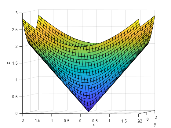
Here is a picture of the boundary of the cone $ \|[x,y]\|\le z $ for nonnegative z.
[X,Y] = meshgrid(-2:0.1:2);
Z = sqrt(X.^2 + Y.^2);
surf(X,Y,Z)
view(8,2)
xlabel("x")
ylabel("y")
zlabel("z")
Of course, you can scale, translate, and rotate a cone constraint. The formal definition of a general cone constraint uses a matrix Asc, vectors bsc and d, and scalar gamma with the constraint in x represented as
norm(Asc*x - bsc) <= d'*x - gamma;
The coneprog solver in Optimization Toolbox requires you to use the secondordercone function to formulate cone constraints. For example,
Asc = diag([1,1/2,0]);
bsc = zeros(3,1);
d = [0;0;1];
gamma = 0;
socConstraints = secondordercone(Asc,bsc,d,gamma);
f = [-1,-2,0];
Aineq = [];
bineq = [];
Aeq = [];
beq = [];
lb = [-Inf,-Inf,0];
ub = [Inf,Inf,2];
[x,fval] = coneprog(f,socConstraints,Aineq,bineq,Aeq,beq,lb,ub)
It can be simpler to use the problem-based approach to access cone programming. This functionality was added in R2021a. For the previous example using the problem-based approach:
x = optimvar('x',3,"LowerBound",[-Inf,-Inf,0],"UpperBound",[Inf,Inf,2]);
Asc = diag([1,1/2,0]);
prob = optimproblem("Objective",-x(1)-2*x(2));
prob.Constraints = norm(Asc*x) <= x(3);
[sol,fval] = solve(prob)
Notice that, unlike most nonlinear solvers, you do not need to specify an initial point for coneprog. This comes in handy in the following example.
Discrete Dynamics With Cone Constraints
Suppose that you want to control a rocket to land gently at a particular location using minimal fuel. Suppose that the fuel used is proportional to the applied acceleration times time. Do not model the changing weight of the rocket as you burn fuel; we are supposing that this control is for a relatively short time, where the weight does not change appreciably. There is gravitational acceleration g = 9.81 in the negative z direction. There is also linear drag on the rocket that acts in the negative direction of velocity with coefficient 1/10. This means after time t, without any applied acceleration or gravity, the velocity changes from v to $ v\exp(-t/10) $.
In continuous time the equations of motion for position $ p(t) $, velocity $ v(t) $, and applied acceleration $ a(t) $ are
$ \frac{dp}{dt} = v(t) $
$ \frac{dv}{dt} = -v(t)/10 + a(t) + g*[0,0,-1] $.
Here are some approximate equations of motion, using discrete time with N equal steps of length $ t = T/N $:
$ p(i+i) = p(i) + t*(v(i) + v(i+1))/2 $ (trapezoidal rule)
$ v(i+1) = v(i)*\exp(-t/10) + t*(a(i) + g*[0, 0, -1]) $ (Euler integration).
Therefore,
$ p(i+1) = p(i) + t*v(i)*(1 + \exp(-t/10))/2 + t^2*(a(i) + g*[0, 0, -1])/2 $.
Now for the part that leads to cone programming. Suppose that the applied acceleration at each step is bounded by a constant Amax. These constraints are
$ \|a(i)\| \le {\rm Amax} $ for all i.
The cost to minimize should be the sum of the norms of the accelerations times t. Cone programming requires the objective function to be linear in optimization parameters. You can reformulate this cost to be linear by introducing new optimization variables s(i) that are subject to a new set of cone constraints:
$ {\rm cost} = \sum s(i)*t $
$ \|s(i)\| \le a(i) $.
Suppose that the rocket is traveling initially at velocity $ v0 = [100,50,-40] $ at position $ p0 = [-1000,-800,1200] $. Calculate the acceleration required to bring the rocket to position $ [0,0,0] $ with velocity $ [0,0,0] $ at time $ T = 40 $. Break up the calculation into 100 steps ($ t=40/100 $). Suppose that the maximum acceleration $ \rm{Amax} = 2g $.
The makeprob function at the end of this script accepts the time T, initial position p0, and initial velocity v0, and returns a problem that describes the discrete dynamics and cost.
p0 = [-1000,-800,1200];
v0 = [100,50,-40];
prob = makeprob(40,p0,v0)
Set options to solve the cone programming problem using an optimality tolarance 100 times smaller than the default. Use the "schur" linear solver, which can be more accurate for this problem.
opts = optimoptions("coneprog","OptimalityTolerance",1e-8,"LinearSolver","schur");
[sol,cost] = solve(prob,Options=opts)
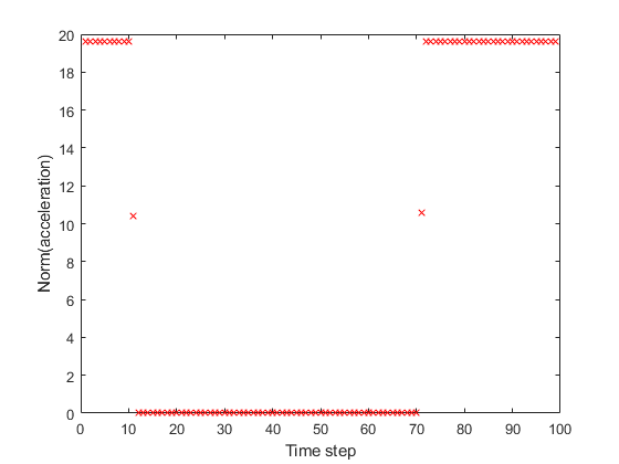
The plottrajandaccel function at the end of this script plots both the trajectory and the norm of the acceleration as a function of time step.
plottrajandaccel(sol)
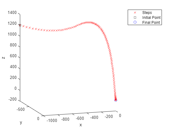
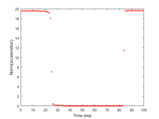
The optimal acceleration is nearly "bang-bang." The rocket accelerates at about $ 2g $ at first, then has close to zero acceleration until the near end. Near the end, the rocket accelerates at maximum to slow the descent and land with zero velocity. The total cost of this control is about 313.
Find Optimal Time
Find the optimal time T for the rocket to land, meaning the time that causes the rocket to use the least possible fuel. The findT function at the end of this script calls fminbnd to locate the minimal-cost time. I experimented briefly to find that [20,60] is a reasonable range for times T for the minimum, and I used those bounds in the fminbnd call. If you take a time much less than 20 you get an infeasible problem:
badprob = makeprob(15,p0,v0);
badsol = solve(badprob,Options=opts)
(As an aside, if you try to make T an optimization variable then the problem is no longer a coneprog problem. Instead, it is a problem for fmincon, which takes much longer to solve in this case, and requires you to provide an initial point.)
Topt = findT(opts)
Plot the optimal trajectory and acceleration.
probopt = makeprob(Topt,p0,v0);
[solopt,costopt] = solve(probopt,Options=opts)
plottrajandaccel(solopt)
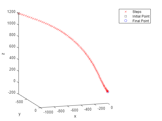
The optimal cost is about 171, which is roughly half of the cost for the original parameters. This time, the control is more nearly bang-bang. The rocket accelerates at maximum at first, then stops accelerating for some time. Again, during the final times the rocket accelerates at maximum to land with zero velocity.
Final Thoughts
Cone programming is a surprisingly versatile framework for solving many convex optimization problems. For another nontrivial example, see Minimize Energy of Piecewise Linear Mass-Spring System Using Cone Programming, Problem-Based. For other problems that can be put in the cone programming framework, see Lobo, Miguel Sousa, Lieven Vandenberghe, Stephen Boyd, and Hervé Lebret. “Applications of Second-Order Cone Programming.” Linear Algebra and Its Applications 284, no. 1–3 (November 1998): 193–228. https://doi.org/10.1016/S0024-3795(98)10032-0
Do you find cone programming or discrete dynamics useful? Do you have any examples of your own to share? Let us know here.
Helper Functions
This code creates the makeprob function.
function trajectoryproblem = makeprob(T,p0,v0)
N = 100;
g = 9.81;
pF = [0 0 0];
Amax = 2*g;
p = optimvar("p",N,3);
v = optimvar("v",N,3);
a = optimvar("a",N-1,3);
s = optimvar("s",N-1,"LowerBound",0,"UpperBound",Amax);
trajectoryproblem = optimproblem;
t = T/N;
trajectoryproblem.Objective = sum(s)*t;
scons = optimconstr(N-1);
for i = 1:(N-1)
scons(i) = norm(a(i,:)) <= s(i);
end
acons = optimconstr(N-1);
for i = 1:(N-1)
acons(i) = norm(a(i,:)) <= Amax;
end
vcons = optimconstr(N+1,3);
vcons(1,:) = v(1,:) == v0;
vcons(2:N,:) = v(2:N,:) == v(1:(N-1),:)*exp(-t/10) + t*(a + repmat([0 0 -g],N-1,1));
vcons(N+1,:) = v(N,:) == [0 0 0];
pcons = optimconstr(N+1,3);
pcons(1,:) = p(1,:) == p0;
pcons(2:N,:) = p(2:N,:) == p(1:(N-1),:) + (1+exp(-t/10))/2*t*v(1:(N-1),:) + t^2/2*(a + repmat([0 0 -g],N-1,1));
pcons((N+1),:) = p(N,:) == pF;
trajectoryproblem.Constraints.acons = acons;
trajectoryproblem.Constraints.scons = scons;
trajectoryproblem.Constraints.vcons = vcons;
trajectoryproblem.Constraints.pcons = pcons;
end
This code creates the plottrajandaccel function.
function plottrajandaccel(sol)
figure
psol = sol.p;
p0 = psol(1,:);
pF = psol(end,:);
plot3(psol(:,1),psol(:,2),psol(:,3),'rx')
hold on
plot3(p0(1),p0(2),p0(3),'ks')
plot3(pF(1),pF(2),pF(3),'bo')
hold off
view([18 -10])
xlabel("x")
ylabel("y")
zlabel("z")
legend("Steps","Initial Point","Final Point")
figure
asolm = sol.a;
nasolm = sqrt(sum(asolm.^2,2));
plot(nasolm,"rx")
xlabel("Time step")
ylabel("Norm(acceleration)")
end
This code creates the fvalT function, which is used by findT.
function Fval = fvalT(T,opts)
p0 = [-1000,-800,1200];
v0 = [100,50,-40];
tprob = makeprob(T,p0,v0);
opts = optimoptions(opts,"Display","off");
[~,Fval] = solve(tprob,Options=opts);
end
This code creates the findT function.
function Tmin = findT(opts)
disp("Solving...")
Tmin = fminbnd(@(T)fvalT(T,opts),20,60);
disp("Done")
end
Copyright 2021 The MathWorks, Inc.
- Category:
- New Feature,
- Optimization


Comments
To leave a comment, please click here to sign in to your MathWorks Account or create a new one.