Loren on the Art of MATLAB

July 17th, 2008

Interpolating Polynomials

John D'Errico is back today to talk about interpolating polynomials.

Contents

Introduction

I talked in my last blog about polynomial regression models. We saw some utility in polynomial models, and that increasing the order of the polynomial caused the errors to decrease. How far can we go? Can we reduce the errors to zero?

At some point, I might choose to increase the degree of the polynomial to one less than the number of data points. Assuming that my data have no replicated points, this is an interpolating polynomial that fits our data exactly, at least to within the double precision accuracy of our computations. A straight line can pass through any two points, a quadratic passes through three points, a cubic hits four points exactly, etc. If you prefer to think in terms of statistical degrees of freedom, if you have n points, a polynomial of order n-1 (with n coefficients) passes through your data exactly.

I've started this all out by talking about polynomial modeling in a least squares sense, or regression analysis. But really, I wanted to talk about interpolation, as opposed to the approximations provided by polynomial regression. Perhaps this was an indirect approach, but one of the things I feel important is to distinguish interpolation from the more general modeling/curve fitting tools used in mathematics. This difference is often unappreciated by many users of MATLAB.

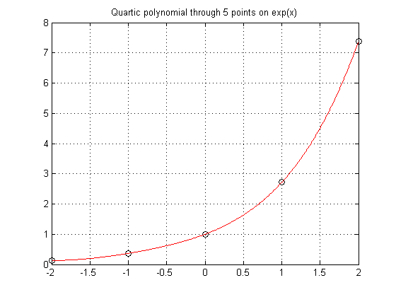
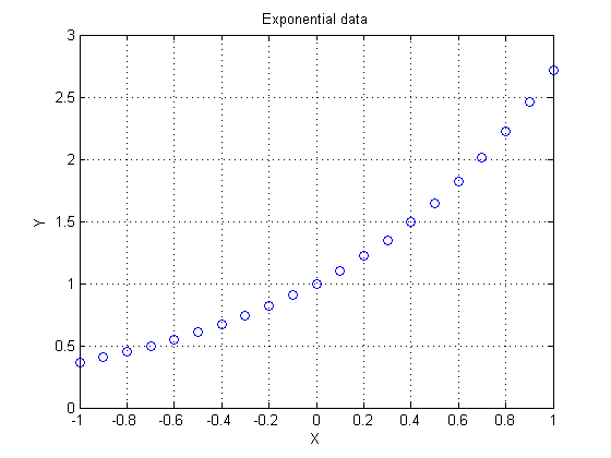
Let's start by sampling five points from an exponential function.

format short
x = (-2:1:2)';
y = exp(x);
plot(x,y,'o')
grid on

Exact Fit

While it is true that polyfit gives an exact fit with an order n-1 polynomial, a direct method is more efficient.

Build an interpolating polynomial using vander coupled with the use of backslash.

P = vander(x)\y
xev = linspace(-2,2,500)';
yev = polyval(P,xev);

plot(x,y,'ko',xev,yev,'r-')
grid on
title('Quartic polynomial through 5 points on exp(x)')
P =
    0.0492
    0.2127
    0.4939
    0.9625
    1.0000

Many books teach you to use the Lagrange form for interpolation. I won't get into that here because I don't really advise the use of polynomials in general.

Interpolation should yield zero residuals at the data points

Verify that the residuals are essentially zero at the data points.

format long g
pred = polyval(P,x) - y
pred =
    -1.11022302462516e-016
    -1.11022302462516e-016
                         0
                         0
                         0

Does the Data Have Replicates?

Suppose I have two points with the same independent variable value, but distinct values for the dependent variable? Since for any given x, a single-valued function returns only a single value for the prediction, this must cause a problem. In this example, what value should I expect for an interpolant when x = 2? Should f(x) be 3 or 4?

x = [0 1 2 2 3 4]';
y = [1 2 3 4 5 6]';
plot(x,y,'-o')

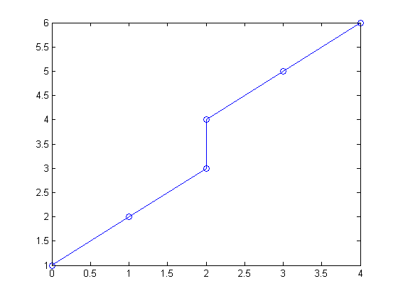
You can see a hint of the problem if you look at the rank of the Vandermonde matrix. The rank should have been 6, but the replicated point causes a singularity.

rank(vander(x))
ans =
     5

This singularity results in a rather useless polynomial.

P = vander(x)\y
Warning: Matrix is singular to working precision.
P =
   NaN
   NaN
   NaN
  -Inf
   Inf
     1

Average the Replicates

If the data truly is not single-valued, the common approach is to use a parametric relationship. (This is something to save for a possible future blog.)

Much of the time however, I just want to do something simple, like average the replicate points. consolidator, a tool I contributed to the File Exchange, can do just that. If you've never found or looked at the file exchange, please take some time to wander through the great tools there.

High Order Polynomials Not a Sure Bet

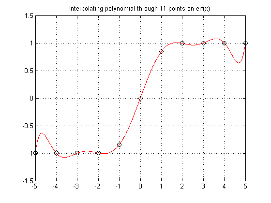
Sometimes polynomials don't do so well. It is important to know your data, know your problem. Here the data comes from a function known to be monotone increasing. Polynomials don't like to be monotone, so forcing a high order polynomial to interpolate such a function is a sure way to fail.

x = (-5:1:5)';
y = erf(x);

P = vander(x)\y
xev = linspace(-5,5,1000)';
yev = polyval(P,xev);

plot(x,y,'ko',xev,yev,'r-')
grid on
title('Interpolating polynomial through 11 points on erf(x)')
P =
     3.49245965480804e-020
      2.0991424886728e-005
    -1.58112816820803e-018
      -0.00119783140998794
     2.17562811018059e-017
        0.0239521737329468
    -9.91270557701033e-017
        -0.211403900317105
     1.85037170770859e-016
          1.03132935951897
                         0

Runge's Phenomenon

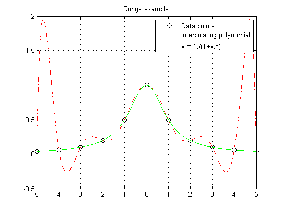
Runge found this example of a function that causes high order interpolating polynomials to fare very poorly.

x = (-5:1:5)';
y = 1./(1+x.^2);
P = vander(x)\y
xev = linspace(-5,5,1000)';
yev = polyval(P,xev);
ytrue = 1./(1+xev.^2);

plot(x,y,'ko',xev,yev,'r-.',xev,ytrue,'g-')
legend('Data points','Interpolating polynomial','y = 1./(1+x.^2)')
grid on
title('Runge example')
P =
    -2.26244343891403e-005
     1.04238735515992e-019
       0.00126696832579186
    -4.47734652027112e-018
       -0.0244117647058824
     5.61044648135202e-017
          0.19737556561086
    -2.38551402729053e-016
         -0.67420814479638
     1.38777878078145e-016
                         1

Numerical Problems

You also need to worry about numerical issues in high order polynomial interpolants. The matrices you would create are often numerically singular.

For example, the rank of the matrix vander(1:n) should be n. However, this fails when working in finite precision arithmetic.

rank(vander(1:10))
rank(vander(1:20))
rank(vander(1:30))
ans =
    10
ans =
     7
ans =
     6

Centering and scaling your data can improve the numerical performance of a high order polynomial to some extent, but that too has a limit. You are usually better off using other interpolation methods.

What can you do? You want to be able to interpolate your data. Polynomials seem like a good place to look, but they have their issues. High order polynomial interpolation often has problems, either resulting in non-monotonic interpolants or numerical problems. You might consider other families of functions to build your interpolant, for example trig or bessel functions, or orthogonal polynomials. Much depends on the relationship you want to model. KNOW YOUR PROBLEM!

By the way, for those who are interested in the methodology of modeling and curve fitting, I list a few ideas in this thread that should be of interest.

We can still do much with polynomials however. They form the basis for many modeling tools.

A nice trick is to go simple. Why use a single high order polynomial to interpolate our data? Instead, break the problem up and use smaller segments of low order polynomials, pieced together. In my next blog I'll begin talking about these piecewise interpolants. Until then please tell me here where you have found interpolating polynomials of use, or if you have found problems that they cannot solve.


Get the MATLAB code

Published with MATLAB® 7.6

19 Responses to “Interpolating Polynomials”

  1. Pavlo replied on :

    Great Post!

    I often use parametric parametrization myself for duplicates. As well I am strongly advocating splines instead of polynomial. Runge-like effects are non-existent there.

  2. Daniel Armyr replied on :

    Hi.
    Our company has a product that uses laser triangulation to measure distance. Unfortunately, the analytical solution to the geometrical problem is numerically highly unstable (many very small angles). Fitting a polynomial to the calibration data also proved difficult as the relationship is very non-polynomial. Higher order polynomials also proved difficult as mentioned in the blog. Piecewise curves was also out of the question due to limited space to store calibration parameters.

    The solution? We inverted one of the parameters and suddenly the curve became very well-behaved and a 6th-order polynomial did the trick nicely.

    The lesson: Don’t be afraid to transform your data before fitting to curves.

  3. John DErrico replied on :

    Pavlo -

    I also strongly recommend splines. But polynomials are the starting point for much that will follow, so they make up my first two blogs here.

    Ringing effects can be significant with splines, but all important is the general shape of the curves you tend to see. At Eastman Kodak, where we used interpolation tools for film and paper response curves, almost all curve shapes tend to have a horizontal lower and upper asymptote, where any ringing will show up easily. So a polynomial model would be terrible, but so would a standard cubic spline. Tools like pchip are necessary there.

  4. John DErrico replied on :

    Daniel -

    Inverse models are very important. When I taught classes in splines and curvefitting techniques, one of the examples I used was a simple one. Suppose you wish to fit the function

    y = sqrt(x)

    for x >= 0. Near zero, the curve has a derivative singularity, so any polynomial model will be a poor choice. As well, a cubic spline is poor in that vicinity too, since it too will be made of cubic segments.

    On the other hand, switch the dependent and independent variables, and the curve is obviously very easily modeled using a low order polynomial, x = y^2. Sometimes there is an issue that when you switch the variables, you are left with an errors in variables problem, so you must beware. But small amounts of noise may not hurt you too much.

    This also points out one important thing. All of my splines evaluation utilities always have had the ability to evaluate the inverse of a spline for any value, i.e., solve for the value of x such that f(x) = y0 for some given y0.

  5. Quan replied on :

    Great tutorial. The MATLAB functions are only as useful as you make them to be. Knowing your data is key. Are splines usually the way to go when interpolating data? If so, what kind of splines are the best bet? I know there are a bunch of options within MATLAB.

  6. John DErrico replied on :

    “Knowing your data is key.” Absolutely true. Understand the system that you are modeling. The more information that you can bring to the modeling process, the better may be your result.

    Very important also is understanding the interpolation tools you will use. A spline is often a good choice, I’d suggest they are usually a better choice than interpolating polynomials. The problem with a high order polynomial is it is not easy to control their shape. But I can do very much with splines, in terms of monotonicity, curvature, etc. If you really need an extra order of differentiability, then you might go up in order, perhaps to a quintic spline. Of course then it becomes harder to control the shape of the curve.

    There are a few variations of splines to be found in interp1, the piecewise linear interpolant, a standard cubic spline, pchip, and the version 5 cubic. I’ll start discussing the differences between these alternatives in my next couple of blogs.

    As well, it is sometimes useful to transform your data before a spline fit. For example, suppose your curve represents the spectral power function of an illuminant. As such, you know that it can never go less than zero, so your interpolant too should always be positive. But the traditional spline is not terribly easy to be constrained for positivity, and very often it might predict negative values. And while pchip is an option here, since it will not introduce new extrema into the curve that did not originally exist, I’ve found that pchip is often a poor choice for this class of curve. (It is often a very poor choice for a spiky fluorescent illuminant.) The problem is you are interpolating in the wrong domain. Transform your data, taking the log of it. Now perform the interpolation using a simple cubic spline, and then convert back by exponentiation to the original space. This absolutely ensures positivity, and does so very simply.

    John

  7. sundar replied on :

    Hello,

    I want to interpolate a data set with spline of higher order ( say 5th order ).
    since spline command can only do cubic spline inerpolation, can you pl. help in doing this?

    Regards,
    Sundar.

  8. John DErrico replied on :

    Sundar - use the splines toolbox to do higher order interpolation than a cubic. For example,

    x = 0:1:20;
    y = sin(x/2);
    spl = spapi(6,x,y);

    The result is a quintic spline, composed of 5th degree polynomial segments. You can convince yourself of that by plotting the 5th derivative of this function, which must be piecewise constant.

    fnplt(fnder(spl,5))

    John

  9. sundar replied on :

    John DErrico ,

    Thanks a lot for your reply.

    This is giving only one set of coeffs. unlike ’spline’ function.
    I think spapi is generating only one polynomial fitting all the data.
    Is there any way thru which I can generate similar piecewise polynomials which is of higher order.

    Can you help me on this pl.

    Regards,
    Sundar.

  10. John DErrico replied on :

    Sundar - see the example I gave before.

    x = 0:1:20;
    y = sin(x/2);
    S = spapi(6,x,y)
    S =
    form: ‘B-’
    knots: [0 0 0 0 0 0 3 4 5 6 7 8 9 10 11 12 13 14 15 16 17 20 20 20 20 20 20]
    coefs: [1×21 double]
    number: 21
    order: 6
    dim: 1

    Note that the form is shown as ‘B-’, as opposed to ‘pp’. Plot the 5th derivative of this function.

    fnplt(fnder(spl,5))

    That derivative plot is piecewise constant. The function is NOT a single polynomial. This is a spline, composed of quintic polynomial segments. The coefficients of the spline are just not represented in the same pp form that spline produces.

    spline(x,y)
    ans =
    form: ‘pp’
    breaks: [0 1 2 3 4 5 6 7 8 9 10 11 12 13 14 15 16 17 18 19 20]
    coefs: [20×4 double]
    pieces: 20
    order: 4
    dim: 1

    John

  11. sundar replied on :

    John DErrico ,

    Thanks again.

    1. In that case, if I need the coefs. of those piecewise quintic curves, how can i get it?. This is reqd. for some manual derivation purposes.
    2. How spapi fn. will determine the knot sequence for a given set of data.

    thanks,
    -sundar

  12. John DErrico replied on :

    Sundar - the easiest way to convert the result into a pp form is this:

    function pp = B2PP(Bform)
    % converts spapi created spline form to a pp form
    % pp = B2PP(Bform)
    breaks = unique(Bform.knots);
    x = breaks(1:(end-1))’;
    n = Bform.order;
    coef = zeros(length(x),n);
    for i = 1:n
    coef(:,n-i+1) = fnval(Bform,x)/factorial(i-1);
    Bform = fnder(Bform);
    end
    pp = mkpp(breaks,coef);

    John

  13. sundar replied on :

    John DErrico ,
    Thanks for that.

    I need to generate a closed spline i.e. when I plot theta (independent variable) against radius (dependent variable) in polar graph, I should get a continuous spline curve.

    Using spapi(), if I give 1st data point again as last one to make it a closed one,I am not getting smooth curve at this closing point. Even if I repeat the second point, result is a distorted spline instead of a smooth one.

    I need to do this for quintic and cubic splines.

    Can you pl. help on this. Thanks in advance.

    -Sundar

  14. rSekuler replied on :

    John: Can you recommend an approach to this possibly-unusal problem? I have data sets in which y=k over some interval (x<n), after which there is a fairly abrupt change to y=mx. The value of n at which the change occurs varies over conditions, and I need to estimate best fitting value of n for each data set.

  15. Vic replied on :

    Hi,

    I’m trying to fit a spline through non distinct data. I know parametrising is the way to go because the repeated values are important. However im not sure how to efficiently parametrise the data points i have in order to fit a cubic spline through it. Any ideas or help would be greatly appreciated.

    Vic

  16. John DErrico replied on :

    Vic,

    Normally when you have non-distinct data points, the answer is to average them. Interpolating splines simply cannot yield two different values of y (the dependent variable) for the same x (independent variable.)

    So the traditional response is to average. the y for replicate x. My consolidator code was written for this purpose (on the File Exchange.)

    It sounds like you have a relationship where this fails. This can happen when you try to interpolate data points around the perimeter of a circle, for example. Here we have a perfectly simple relationship, but where the interp1 type of spline interpolant will fail miserably. The trick is to use a parametric interpolant, as you alluded to. This is done in cscvn, from the splines toolbox, but you can easily do it yourself.

    Here is an example:

    xy = randn(20,2);
    r = sqrt(sum(xy.^2,2));
    x = xy(:,1)./r;
    y = xy(:,2)./r;
    plot(x,y,'o')
    

    As you can see, these points lie on the circumference of a circle. I’ll sort them, based on angle.

    theta = atan2(y,x);
    [theta,tags] = sort(theta);
    x = x(tags);
    y = y(tags);
    

    Wrap around, since we want our interpolant to be around a full circle.

    x = [x;x(1)];
    y = [y;y(1)];
    plot(x,y,'o-')
    

    As you surely see, the piecewise linear interpolant here is poor. There will be some big sectors of the circle that are poorly approximated by only 20 random points. The trick is to use piecewise linear chord length to parameterize on. Yeah, I know that sounds impressive. but can I write it in one line of code? (Yes.) In fact, I’ve always thought this was kind of pretty.

    t = cumsum(sqrt(([0;diff(x)].^2 + [0;diff(y)].^2)));
    plot(t,x,'r-o',t,y,'b-s')
    

    It should not surprise you that these two curves look vaguely trigonometric. Can we use it though?

    tinterp = linspace(t(1),t(end),1000);
    xinterp = interp1(t,x,tinterp,'spline');
    yinterp = interp1(t,y,tinterp,'spline');
    plot(xinterp,yinterp,'r-')
    hold on
    plot(x,y,'bo')
    hold off
    grid on
    axis equal
    

    If I do say so myself, this is not a bad circular interpolant. Ok, there will be someone in the peanut gallery who will point out that this interpolant is not perfect, because it need not be differentiable across the wrap point. Recall that I used the basic spline from interp1, which employed not-a-knot end conditions. Had I used a spline with periodic end conditions, I would have gotten a somewhat better result. A simple trick, if you don’t want to go through the effort of building/finding an interpolating spline with periodic end conditions, is to wrap several points around each end of the spline. This will get you closer to periodicity without making any serious mental effort.

    These arc length parameterized splines are nice, because they work as well in higher dimensions.

    John

  17. Zoh replied on :

    Hello,

    I am currently working on the matlab spline toolbox in order to describe a specific movement. I have two question:

    Using a cubic spline function, how can we specify the condition at the interior points, (i want to have a straight horizontal line between two of the interior points, i imagine it could be possible by defining zero slopes at these two points or by joining different splines).

    can anybody help ???

    thanks in advance

    Zohaib

  18. John DErrico replied on :

    Hi Zohaib,

    I saw your question on the newsgroup, and decided that the best solution was something I had to finish writing before I could respond. It is now at a realistic stage to reply, and to post on the file exchange. It should appear on Monday.

    I’ve written a set of tools called by the acronym SLM, for “Shape Language Modeling”. These represent a way of doing modeling that uses a set of shape primitives, prescribed in advance by the user. The idea is that a scientist/engineer/analyst/modeler often has specific knowledge about their process. This knowledge may come from some basic physical understanding of the system they are modeling, it may come from word of mouth, it may be an observation made from past experience about similar data, or even just from looking at a plot of the data. Regardless, these pieces of information are not always trivial to implement as part of the curve fitting process.

    For example, a frequent piece of information about a curve is that it must be monotone. Perhaps your process is such that physical argument tells you it must always be a monotonic increasing function? Your data may have noise in it so that it is bumpy, but in your head you know that is MUST be monotone and increasing. Usually what happens is the person doing the curve fit will find a nonlinear regression model to fit the data that happens to be monotone and increasing. In fact, I’ll argue that this is the single biggest reason why people use these nonlinear regression models. They use various sigmoid functions, erfs, etc. In fact, I list several such different increasing curve shapes in my Nonlinear Regression Shapes submission on the file exchange.

    http://www.mathworks.com/matlabcentral/fileexchange/10864

    My point is that people often do nonlinear regression not because they want to do so, but because they are forced to do so, because they wish to build some piece of information into their curve to be fit. While monotonicity is the most common shape primitive that people seem to want to use, there are many others. For example, suppose you wished to estimate an MTF (Modulation Transfer Function) curve from some measured data points. Much of the time it is assumed that at a frequency of 0, the modulation is at 100%. So the curve must pass through the point [0,1] in the plot. Furthermore, you might wish to assume other information about the process, perhaps that the modulation will not go above 100%, or that it will never be a negative number.

    Some other common shape primitives might be that the function has everywhere a positive (or negative) second derivative, or that the function is locally constant over some internal range. (This last is the question that you have asked about.) You may also wish to employ periodicity in your model, or specify that the function has a single peak in some area, but then drop off away from that point.

    Given noisy data however, the data may drive a curve fit by a simple least squares spline or polynomial to do strange things however, that contradict these pieces of intrinsic knowledge that you may have. How do you force the curve to do what you know in your mind must happen, yet still fit the data as best as possible?

    The solution is to provide a curve fitting tool that allows you to build any shape primitives into the model itself, in terms of a natural language of shape primitives. I do this using splines. The tool is called slmengine, because it will be the computational engine behind the SLM tools. The slmengine tool allows commandline input to describe the shape of your model. The part of these tools that is not yet fully written is a graphical front end that will allow a direct interface to these tools. In the meantime, I’ll post what I have written, as these tools are now at a fully useable and documented stage.

    I’ll give a few examples of how you might use these tools here. I’ll create some data that has an interesting shape.

    x = (sort(rand(1,100)) - 0.5)*pi;
    y = sin(x).^5 + randn(size(x))/25;
    plot(x,y,'o')
    

    You can see that the curve has a fair amount of noise in it. Obviously, we know the function must be monotone, given the way I’ve created the curve itself. Suppose we did not know that underlying model? A common solution here is to employ a nonlinear regression as I said before. A BETTER solution is to use my shape language modeling tools. The slmengine tool has a property/value pair interface. (I’m sorry that I cannot actually show you these plots from this response window, because they are instructive.)

    slm = slmengine(x,y,'plot','on','knots',10)
    slm =
                form: 'slm'
              degree: 3
               knots: [10x1 double]
                coef: [10x2 double]
        prescription: [1x1 struct]
                   x: [100x1 double]
                   y: [100x1 double]
    

    This returns the cubic spline in a Hermite form. It has 10 knots/breaks. I could also have specified a pp form as the result.

    pp = slmengine(x,y,'plot','on','knots',10,'result','pp')
    pp =
                form: 'pp'
              breaks: [-1.5334 -1.1988 -0.86411 -0.52947 -0.19482 0.13983 0.47447 0.80912 1.1438 1.4784]
               coefs: [9x4 double]
              pieces: 9
               order: 4
                 dim: 1
        prescription: [1x1 struct]
    

    In either case, the result contains a “prescription” field. This contains all of the information that was indicated when we built the spline. It is useful for future reference. You can also get a hint about the possible things one can specify about the shape of your curve.

    slm.prescription
    ans =
                        C2: 'on'
               ConcaveDown: 'off'
                 ConcaveUp: 'off'
            ConstantRegion: []
                Decreasing: 'off'
                    Degree: 3
             EndConditions: 'estimate'
                  Envelope: 'off'
                  ErrorBar: []
                Increasing: 'off'
                  Integral: []
             InteriorKnots: 'fixed'
                     Knots: 10
              LeftMaxSlope: []
              LeftMaxValue: []
              LeftMinSlope: []
              LeftMinValue: []
                 LeftSlope: []
                 LeftValue: []
              LinearRegion: []
                  MaxSlope: []
                  MaxValue: []
                  MinSlope: []
                  MinValue: []
        NegativeInflection: []
                     Order: []
                      Plot: 'on'
        PositiveInflection: []
            Regularization: 0.0001
                    Result: 'pp'
             RightMaxSlope: []
             RightMaxValue: []
             RightMinSlope: []
             RightMinValue: []
                RightSlope: []
                RightValue: []
                   Scaling: 'on'
                SimplePeak: []
              SimpleValley: []
                 Verbosity: 0
                   Weights: []
                        XY: []
                       XYP: []
                      XYPP: []
    

    The slm form of our model can be used by some other tools I supply in this toolkit.

    plotslm(slm)
    

    will plot the spline, giving you a nice graphical interface to look at the derivatives, as well as plot the data on top of it if desired. I also give you tools to evaluate a spline, its derivatives, integrate the spline, etc. All of this is covered in great detail in a tutorial that I’ve written.

    Back to our original curve, the basic call we used before specified that the final result be plotted. Furthermore, the spline will have 10 knots, equally spaced over the span of the data. A better curve fit results from adding more information.

    slm = slmengine(x,y,'plot','on','knots',10,'increasing','on');
    

    Amazingly, this curve is now quite smooth. Simply providing information about the process and building it into your model is quite simple, as I hope you can see here. Here I’ve now added two more pieces of information, i.e., that the left and right hand end point slopes are exactly zero.

    slm = slmengine(x,y,'plot','on','knots',10,'increasing','on','leftslope',0,'rightslope',0);
    

    I can go on further. Suppose I decided that the curve was not quite flat enough in the central region for my purposes. For example, evaluate the second derivative at a few points near zero.

    slmeval([-.2 0 .2],slm,2)
    ans =
        -0.029646  -1.7287e-14     0.035005
    

    Perhaps I want the curve to be constant over that interval? This is what you have asked for, after all.

    slm = slmengine(x,y,'plot','on','knots',10,'increasing','on','leftslope',0,'rightslope',0,'constantregion',[-.2,.2])
    

    See that the second derivative is indeed flat in the vicinity of x = 0.

    slmeval([-.2 0 .2],slm,2)
    ans =
      -5.7416e-15   1.6138e-15  -1.0432e-15
    

    Alternatively, we can look at the maximum and minimum values of the slope over that interval.

    slmpar(slm,'maxslope',[-.2,.2])
    ans =
       3.1475e-16
    
    slmpar(slm,'minslope',[-.2,.2])
    ans =
      -4.1045e-16
    

    I hope that this toolkit is of use to you. I will argue that it will be so for many users of curve fitting, since it allows them to build models for their systems with the intrinsic shapes they know must be present. I am sorry that it took a few days for me to get this up on the file exchange for you. I did want to finish up a few things. As I said above, the slm toolkit should appear on the File Exchange on Monday, 6/15/09. Once it is up, I will plan on making many enhancements over the coming weeks, since I expect to see very much feedback on these tools. I’ll also be cleaning up any minor problem that surely will surface.

    The SLM toolkit does not require the splines toolbox, although it does use the optimization toolbox because of the class of problems that it forms internally. Really, it mainly uses the function lsqlin, although some rare problems employ other optimizers from that toolbox.

    John D’Errico

  19. Zohaib replied on :

    Thanx John for such a detailed reply….I am grateful for this effort. This helped me a lot.

Leave a Reply

Wrap code fragments inside <pre> tags, like this:

<pre class="code">
a = magic(3);
sum(a)
</pre>

If you have a "<" character in your code, either follow it with a space or replace it with "&lt;" (including the semicolon).


Loren Shure works on design of the MATLAB language at The MathWorks. She writes here about once a week on MATLAB programming and related topics.

  • Jun: I totally can not believe it, Loren. You are really helpful. Thank you so much, MATLAB master!
  • Loren: Wow folks- Always lots of interest when there’s a quickie to try out! I will only make 2 general...
  • Loren: Jun- ismember is your friend here: >> [aa,ind] = ismember(Array2,Arra y1) aa = 1 1 1 1 1 1 1 ind = 1 2 1 4 4 3...
  • Dan: I like the first way better than the second way. Combining the arrays into one and running any is nice, although...
  • James Myatt: How about I = (a == 0 | b == 0); a(I) = []; b(I) = [];
  • Tunc: Hello Loren, love your blog because of such inspiring and challenging comments to such ’small’...
  • Pekka Kumpulainen: Here is my tradeoff. I usually want to keep the original variables as they are most probably...
  • Iain: Followup: Of course, to allow NaNs (counting them as non-zero): mask = (a~=0) & (b~=0); The mask says “a...
  • Matt Fig: I would usually go with something like this: y = a&b; x = a(y); y = b(y); But I was surprised to find...
  • kk: c=all([a;b]) a(c) a(b)

These postings are the author's and don't necessarily represent the opinions of The MathWorks.