
MathWorks Logo, Part Four, Method of Particular Solutions Generates the Logo
The Method of Particular Solutions computes a highly accurate approximation to the eigenvalue we have been seeking, and guaranteed bounds on the accuracy. It also provides flexibility involving the boundary conditions that leads to the MathWorks logo.

 So this is actually the first eigenfunction of the L-shaped membrane.
 This function is an exact solution of the partial differential equation
$$ \Delta u + \lambda u = 0 $$
with the value of $\lambda$ reported above. It satisfies the boundary condition $u = 0$ on the two edges meeting at the reentrant corner, but it fails significantly on the outer edges. So it is only with some artistic license that we can refer to it as the first eigenfunction of L-shaped membrane.
When I first saw this surf plot, it didn't have this gorgeous color map, but I found the shape so attractive that I kept it around. The evolution of the shading, lighting and colors that turned this into our logo is the subject of my next blog.
This function is an exact solution of the partial differential equation
$$ \Delta u + \lambda u = 0 $$
with the value of $\lambda$ reported above. It satisfies the boundary condition $u = 0$ on the two edges meeting at the reentrant corner, but it fails significantly on the outer edges. So it is only with some artistic license that we can refer to it as the first eigenfunction of L-shaped membrane.
When I first saw this surf plot, it didn't have this gorgeous color map, but I found the shape so attractive that I kept it around. The evolution of the shading, lighting and colors that turned this into our logo is the subject of my next blog.
Contents
Eidgenossische Technische Hochschule Zurich
In 1965-66, after finishing grad school, I spent a postdoctoral year at the ETH, the Swiss Federal Institute of Technology in Zurich. At the time, the faculty included three world renowned numerical analysts, Eduard Stiefel, Heinz Rutishauser, and Peter Henrici. Moreover, IBM had a branch of their research division in Ruschlikon, a Zurich suburb, where they held occasional seminars. In October, Leslie Fox, from Oxford, visited the IBM center and gave a talk about the work two of his students, Joan Walsh and John Reid, were doing on the L-shaped membrane. Expansions involving Bessel functions that matched the singularity of the eigenfunction near the reentrant corner were coupled to finite difference grids in the rest of the domain. Shortly after Fox's talk, it occurred to me to use the Bessel function expansions over the entire domain and avoid finite differences altogether. Within a matter of weeks I had done computations on the CDC 1604 mainframe at the ETH that had me very excited. To celebrate, I made an L-shaped ornament out of aluminum foil for the Christmas tree in our apartment. Henrici contributed some theoretical background relating what I was doing to work of Stephan Bergman and a Russian mathematician I. N. Vekua. Together with Fox, we published a paper in the SIAM Journal on Numerical Analysis in 1967.Method of Particular Solutions
You don't need to know much about Bessel functions to appreciate the method of particular solutions. Using polar coordinates, a particular solution is any function of the form $$ v_\alpha(\lambda,r,\theta) = B_\alpha(\sqrt{\lambda} r) \sin{(\alpha \theta}) $$ First of all, notice that the $\sin{(\alpha \theta)}$ portion insures that this solution satisfies the boundary condition $$ v_\alpha(\lambda,r,\theta) = 0 $$ along the two rays with $\theta = 0$ and $\theta = {\pi}/{\alpha}$. For our L-shaped domain the reentrant corner has an angle of $\frac{3}{2}\pi$, so we will want to have $$ \alpha = \frac{2}{3}j $$ where $j$ is an integer. The Bessel function $B_\alpha$ is defined by an ordinary differential equation that implies any $v_\alpha$ satisfies the partial differential equation $$ \Delta v_\alpha + \lambda v_\alpha = 0 $$ If $\alpha$ is not an integer, then $B_\alpha(r)$ has another important property. Its derivatives blow up as $r$ goes to 0. This asymptotic singularity is just what we need to match the singularity in the eigenfunction. We can also take advantage of symmetries. The first eigenfunction is symmetric about the centerline of the L. We can also eliminate components that come from the eigenfunctions of the unit squares that are subdomains. This implies that for the first eigenfunction $\alpha = \frac{2}{3}j$ where $j$ is an odd integer that is not a multiple of 3, that is $$ \alpha_j = \frac{2}{3}j, \ \ j = 1,5,7,11,13, ... $$Boundary Conditions
Form a linear combination of particular solutions. $$ u(\lambda,r,\theta) = \sum_\alpha c_\alpha v_\alpha(\lambda,r,\theta) $$ This function satisfies our differential equation throughout the domain, satisfies the boundary condition on the two edges that meet at the reentrant corner, and has the desired singular behavior there. All we have to do is pick $\lambda$ and the coefficients $c_\alpha$ so that $u$ satisfies the boundary condition, $u = 0$, on the remaining edges of the L. The general idea is to pick a number of points on the outer boundary and investigate the matrix obtained by evaluating the particular solutions in the linear combination at these points. Vary $\lambda$ until that matrix is nearly rank deficient. The resulting null vector provides the desired coefficients. The details of how we carry out this general plan have varied over the years. The best approach is implemented in the function membranetx, available here, described in the PDE chapter of Numerical Computing with MATLAB. It uses the matrix computation workhorse, the SVD, the singular value decomposition. The number of rows in the matrix involved is the number of points on the boundary and the number of columns is the number of terms in the sum. The figures below come from matrices that are 46-by-9. Let $(r_i,\theta_i)$ be the points chosen on the boundary. The matrix elements are $$ a_{i,j}(\lambda) = B_{\alpha_j}(\sqrt{\lambda} r_i) \sin{(\alpha_j \theta_i)} $$ The function fmintx is used to vary $\lambda$ and find a minimum of the SVD of this matrix. The resulting matrix is essentially rank deficient and the resulting right singular vector is a null vector that provides the coefficients. The minimum is found at $$ \lambda = 9.639723844 $$ Here are the first four particular solutions. The vertical scale reflects the magnitude of the corresponding coefficient.mps_figs
All Four Terms
None of these four terms is remotely close to zero on the outer boundary, but when they are added together the sum is zero to graphical accuracy.mps_figs(4)
Just Two Terms
Now we can have some fun. Here is a surf plot of the sum of just the first two particular solutions.mps_figs(2)
Upper and lower bounds
The Fox, Henrici and Moler paper was not just about the method of particular solutions. We were also concerned about finding guaranteed upper and lower bounds for the exact eigenvalue of the continuous differential operator. A theorem proved in the paper relates the discrepancy in meeting the boundary condition to the width of a small interval containing the eigenvalue. In 1966 we proved $$ 9.6397238_{05} < \lambda < 9.6397238^{84} $$ Today with membranetx on MATLAB, I am finding a value of $\lambda$ in the center of this interval. [L,lambda] = membranetx(1);
format long
lambda
lambda =
   9.639723844021997


Comments
To leave a comment, please click here to sign in to your MathWorks Account or create a new one.