
How Many Times Should You Shuffle the Cards?
We say that a deck of playing cards is completely shuffled if it is impossible to predict which card is coming next when they are dealt one at a time. So a completely shuffled deck is like a good random number generator. We saw in my previous post that a perfect faro shuffle fails to completely shuffle a deck. But a riffle shuffle, with some randomness in the process, can produce complete shuffling. How many repeated riffle shuffles does that take?
"Stop Shuffling and Deal."
Contents
Background
I learned about this topic from my friend Nick Trefethen, a Professor at Oxford and a MATLAB enthusiast. In 2000 he and his father wrote a paper, "How Many Shuffles to Randomize a Deck of Cards?". They refer to work by Persi Diaconis and colleagues. Diaconis is a Professor at Stanford and a world-class magician who has written extensively about the probability involved in activities like card shuffling and coin flipping.
I want to describe some simulations that reproduce the cutoff phenomenon investigated by the Trefethens and Diaconis.
Rising Sequences
The analysis is based on the number of rising sequences in the shuffled deck. A rising sequence is a maximal subset of cards in increasing numerical order. A deck is the union of its rising seguences. Here is an example, a small deck with just eight cards.
v = [3 1 4 5 7 2 8 6];
There are three rising sequences is this example.
[1 2]; [3 4 5 6]; [7 8];
Signature
We define the signature of a deck to be the number of rising sequences. Here is a tricky, but elegant, way to compute the signature of a deck v. Sort the deck to find the permutation vbar that reverses v, then count the number of places where vbar has a negative first difference.
type signature
   function sig = signature(v);
      [~,vbar] = sort(v);
      sig = sum(diff(vbar)<0)+1;
   end
sigv = signature(v)
sigv =
     3
Let's see how this works on the example.
   [~,vbar] = sort(v)
   d = diff(vbar)<0;
   disp('d = ')
   disp(['   ', sprintf('%6.0f', d)]),
   sig = sum(d)+1
vbar =
     2     6     1     3     4     8     5     7
d =
        0     1     0     0     0     1     0
sig =
     3
Unshuffled Decks
An unshuffled deck of n cards, fresh out of the package, is represented by the vector v = 1:n. This has one long rising sequence, so the signature is 1. If you reverse the order, each card by itself is a singleton rising sequence, so the signature of the deck is n. These are the minimum and maximum possible values for the signature.
   n = 52;
   v = 1:n;
   sig_min = signature(v)
   sig_max = signature(fliplr(v))
sig_min =
     1
sig_max =
    52
Perfect Shuffles
As we saw in my previous post, the "out" perfect shuffle keeps the first and last cards in first and last place, while the "in" perfect shuffle inserts these cards in the second and next-to-last places. Here are their permutation vectors.
   m = n/2;
   pout = reshape([1:m; m+(1:m)],[1,n]);
   pin = reshape([m+(1:m); 1:m],[1,n]);
Both shuffles produce decks with two rising sequences obtained from the two halves of the deck. So their signatures are both equal to 2.
   sig_pout = signature(v(pout))
   sig_pin = signature(v(pin))
sig_pout =
     2
sig_pin =
     2
These signatures for pout and pin are way too small; the presence of just two rising sequences indicates perfect shuffles do not produce completely shuffled results.
Random Permutations
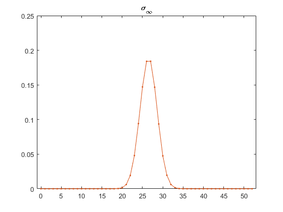
A completely shuffled deck could be obtained by spreading the cards out on the table and then picking them up one at a time in a random order. This would be a random permutation of the integers 1:52. Let's examine the signature of random permutations. We'll generate a million samples, then normalize the histogram of the resulting signatures so that it becomes a probability distribution, $\sigma_\infty$. This is the signature distribution of completely shuffled decks. Our goal is to get close to this distribution with riffle shuffling. (In order to reduce publication time, distributions are computed separately.)
type compute_sigma_inf
    ksamples = 1000000;
    s = zeros(ksamples,1);
    for k = 1:ksamples
       v = randperm(n);
       s(k) = signature(v);
    end
    sigma_inf = hist(s,0:n)/length(s);
    save sigma_inf sigma_inf
    load sigmas_52
    plot(0:n,sigma_inf)
    plot_details_inf
Support
The distribution $\sigma_\infty$ is centered at 26 and 27 and falls off quickly from these two points. Here are the indices and values of all probabilities greater than .005. This tells us that completely shuffled decks have 26 or 27 increasing sequences 18.4% of the time each and that fewer than 21 or more than 32 increasing sequences are very unlikely.
support(sigma_inf,.005)
     21     22     23     24     25     26     27     28     29     30     31     32
 0.0061 0.0193 0.0480 0.0942 0.1471 0.1840 0.1841 0.1467 0.0936 0.0475 0.0196 0.0062
Riffle Shuffle
There are two sources of randomness in this model. The deck is cut at a depth determined by a random number chosen from a binomial distribution centered at its midpoint. Cards are then riffled back together. At each step the probability that the next card drops from either cut is proportional to the size of that cut.
type riffle
    function vout = riffle(v)
    % Riffle Shuffle.
    % vout = riffle(v)

       % Cut deck roughly in half.
       n = length(v);
       m = binornd(n,0.5); % Binomial distribution

       % Interleave cuts.
       vout = zeros(1,n);
       i = 1;
       j = m+1;
       for k = 1:n
          % Choose which cut releases next card.
          % Probability is proportional to size of cut.
          if rand*(n-k+1) < m-i+1
             vout(k) = v(i);
             i = i+1;
          else
             vout(k) = v(j);
             j = j+1;
          end
       end
    end
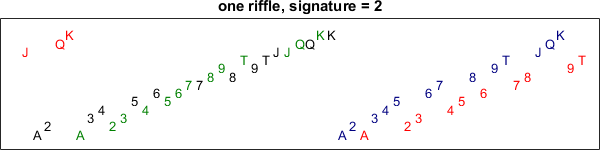
Here is one riffle shuffle of a fresh deck. The result almost certainly has a signature equal to 2, although the signature could be only 1 in the extremely unlikely event that the entire first cut falls in one clump before any of the second cut.
     v = riffle(1:n);
     deck_view(v)
     title(['one riffle, signature = ' int2str(signature(v))])
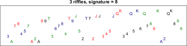
Here are three riffles of a fresh deck. The result is likely to have a signature equal to 8, although any smaller value is possible.
     v = riffle(riffle(riffle(1:52)));
     deck_view(v)
     title(['3 riffles, signature = ' int2str(signature(v))])
     snapnow
     close
Repeated Riffle Shuffles
Find the probability distribution generated by repeating a riffle shuffle r times. Denote this by $\sigma_r$.
type repeated_riffles
    function sigma_r = repeated_riffles(n,r,ksamples)
       % sigma_r = repeated_riffles(n,r,ksamples)
       % Signature distribution of r repeated riffle shuffles.
       s = zeros(ksamples,1);
       for k = 1:ksamples
          v = 1:n;
          for j = 1:r
             v = riffle(v);
          end
          s(k) = signature(v);
       end
       sigma_r = hist(s,0:n)/length(s);
    end
Compute Distributions
For each value r between 0 and rmax, sample the signature $\sigma_r$ observed when a deck is subjected to r repeated riffle shuffles.
     rmax = 14;
     type compute_sigmas
     sigma = zeros(rmax+1,n+1);
     ksamples = 1000000;
     for r = 0:rmax
        sigma(r+1,:) = repeated_riffles(n,r,ksamples)
     end
     save sigmas
load sigmas_52
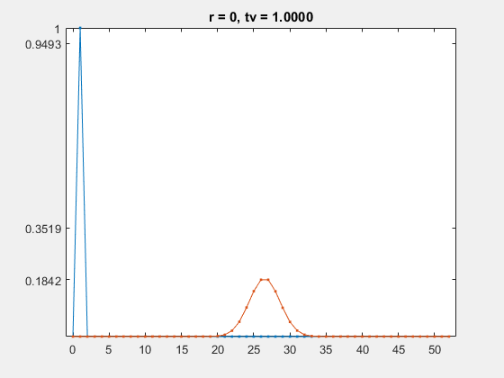
For example, here is $\sigma_3$. Almost 95% of the distribution is concentrated at the maximum signature, 8. Slightly over 5% of the support has a signature in the range of 5 through 7.
     r = 3;
     plot(0:52,sigma(r+1,:),'.-')
     plot_details_r
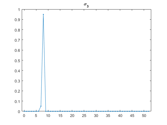
Here is the support of $\sigma_3$.
support(sigma(r+1,:),0)
         5         6         7         8
  0.000001  0.000424  0.050308  0.949267
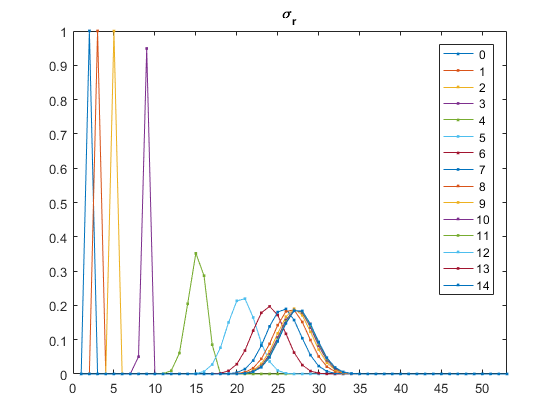
Here are all of the $\sigma_r$. As expected, they appear to be heading towards $\sigma_{\infty}$.
     plot(sigma','.-')
     plot_details_sigma
Total Variation
The total variation norm is a very general concept that measures the distance between two probability distributions. In our situation it is simply the 1-norm of their difference, scaled by 1/2 so that it lies between 0 and 1.
norm_tv =
    @(s1,s2)(1/2)*norm(s1-s2,1)
norm_tv =
@(s1,s2)(1/2)*norm(s1-s2,1)
Total Variation of Repeated Riffles
For each value r between 0 and rmax, sample the signature $\sigma_r$ observed when a deck is subjected to r repeated riffle shuffles. Compare this with the completely shuffled distribution $\sigma_{\infty}$ and compute the total variation.
     tv = zeros(rmax+1,1);
     for r = 0:rmax
        tv(r+1) = norm_tv(sigma(r+1,:), sigma_inf);
     end
     disp('tv =')
     fprintf('%12.6f\n',tv)
tv =
    1.000000
    1.000000
    1.000000
    1.000000
    1.000000
    0.923751
    0.613194
    0.333949
    0.166832
    0.084924
    0.042375
    0.021786
    0.010285
    0.004999
    0.001935
Make an animated gif.
type make_tv_movie
     gif_frame('html/tv_movie.gif');
     for r = 0:rmax
        plot(0:n,[sigma(r+1,:); sigma_inf]','.-')
        plot_details_movie
        gif_frame(2)
     end
     clf
     gif_frame(2)
How many?
How many riffle shuffles are required to produce a completely shuffled deck? Plot the total variation as a function of the number of repetitions. The value of tv hovers very close to 1.0 for the first four shuffles, but then between five and nine shuffles it drops quickly to below 0.1. This is the cutoff phenomenon.
     plot(0:rmax,tv,'o-')
     plot_details_cutoff
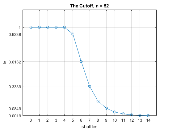
It takes seven shuffles for the total variation to fall below 0.5. The conclusion is that about seven riffle shuffles are usually necessary and sufficient to produce a completely shuffled deck. Diaconis reaches this conclusion with a rigorous probabilistic analysis. Trefethen sees the cutoff with an analysis involving matrix powers and pseudospectra.
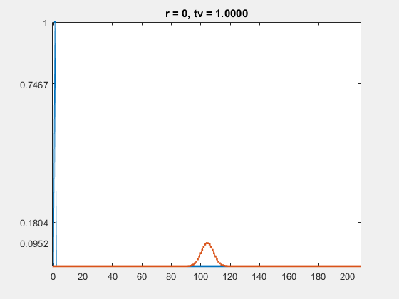
Four decks
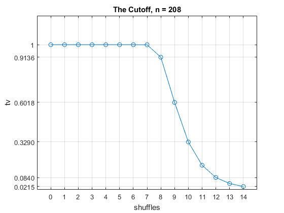
Here are the animation and the cutoff plot for four decks, so n = 208. The distribution of the random permutations, $\sigma_{\infty}$, is more spread out. But the shape of the cutoff is the same, it just occurs three shuffles later.
The conclusion here is that about ten riffle shuffles are usually necessary and sufficient to completely shuffle four decks.
     n = 208;
     load sigmas_208
     disp('tv =')
     fprintf('%12.6f\n',tv)
tv =
    1.000000
    1.000000
    1.000000
    1.000000
    1.000000
    1.000000
    1.000000
    0.999555
    0.913595
    0.601832
    0.328962
    0.168368
    0.083952
    0.042310
    0.021535
     plot(0:rmax,tv,'o-')
     plot_details_cutoff
Acknowledgements
Thanks very much to Nick Trefethen for help with this post.
References
L. N. Trefethen and L. M. Trefethen, "How Many Shuffles to Randomize a Deck of Cards?", Proceedings: Mathematical, Physical and Engineering Sciences 456, 2000. <http://www.jstor.org/stable/2665604>. <http://people.maths.ox.ac.uk/trefethen/publication/PDF/2000_87.pdf>.
Gudbjorn F. Jonsson and Lloyd N. Trefethen, "A Numerical Analyst Looks at the Cutoff Phenomenon in Card Shuffling and Other Markov Chains", Numerical Analysis (ed. D. F. Griffiths, D. J.Higmam and G. A. Watson), Addison-Wesley, 1998. <http://people.maths.ox.ac.uk/trefethen/publication/PDF/1997_74.pdf>.
Dave Bayer and Persi Diaconis, "Trailing the Dovetail Shuffle to its Lair", Annals of Probability 2, 1992. <http://projecteuclid.org/download/pdf_1/euclid.aoap/1177005705>.
A terrific series of videos from an interview with Persi Diaconis on Numberphile.


Comments
To leave a comment, please click here to sign in to your MathWorks Account or create a new one.