 Cleve’s Corner: Cleve Moler on Mathematics and Computing
 The MATLAB Blog
 Guy on Simulink
 MATLAB Community
 Artificial Intelligence
 Developer Zone
 Stuart’s MATLAB Videos
 Behind the Headlines
 File Exchange Pick of the Week
 Hans on IoT
 Student Lounge
 MATLAB ユーザーコミュニティー
 Startups, Accelerators, & Entrepreneurs
 Autonomous Systems
 Quantitative Finance
 MATLAB Graphics and App Building
MATLAB® History, Modern MATLAB, part 1
The ACM Special Interest Group on Programming Languages, SIGPLAN, expects to hold the fourth in a series of conferences on the History of Programming Languages in 2020, see HOPL-IV. The first drafts of papers are to be submitted by August, 2018. That long lead time gives me the opportunity to write a detailed history of MATLAB. I plan to write the paper in sections, which I'll post in this blog as they are available.
This is the fifth such installment and the first of a multipart post about modern MATLAB.
Despite its name, MATLAB is not just a Matrix Laboratory any more. It has evolved over the last 35 years into a rich technical computing environment.
Contents
Graphics
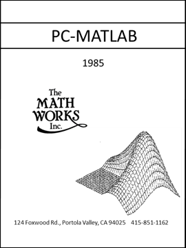
PC-MATLAB had only about a dozen graphics commands, including plot for two-dimensional work and mesh for three dimensions. The results were rendered on low resolution displays with limited memory and few, if any, colors. But as the equipment evolved, so did MATLAB graphics capabilities.
In 1986 we released a version of MATLAB named PRO-MATLAB, for UNIX workstations including the Sun-3. The displays and the window systems on these workstations supported more powerful graphics.
In 1992 we released MATLAB 4 for both PCs and workstations. This release included significant new graphics features, including color. I remember struggling with conversion of the RGB color represention that was the basis for our software to the CMYK representation that was expected by the printers of our paper documention. The problem is under specified. We have three values, R, G and B. They are weighted average of four values, C, M, Y and K. What are those four values? I was immensely pleased when I saw the first successful page proofs for the color insert.
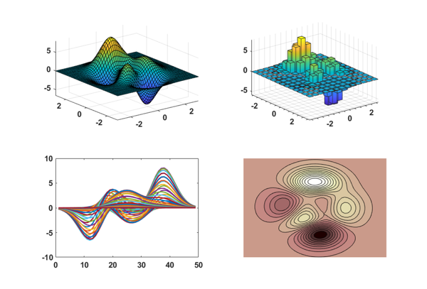
This is not the place to describe all the graphics features we have in MATLAB today. Here's a sample, four different views of one of our venerable test surfaces.
[x,y,z] = peaks;
$$ z = 3(1-x) e^{-x^2-(y+1)^2} -10(\textstyle\frac{x}{5}-x^3-y^5) e^{-x^2-y^2} -\textstyle\frac{1}{3} e^{-(x+1)^2-y^2} $$
%  First, an unadorned surface plot.

   p1 = subplot(2,2,1);
   surf(x,y,z)
   axis tight

% Next, a 3D bar chart, with some adjustment of the default annotation.

   p2 = subplot(2,2,2);
   k = 1:4:49;
   b = bar3(flipud(z(k,k)));
   fixup(p2,b)

% Then, a 2D plot of the columns of the array.

   p3 = subplot(2,2,3);
   plot(z)

% Finally, a filled contour plot with 20 levels and a modest color map.

   p4 = subplot(2,2,4);
   contourf(z,20);
   colormap(p4,pink)
   axis off
Data types
For many years MATLAB had only one numeric data type, IEEE standard 754 double precision floating point, stored in the 64-bit format.
   clear
   format long
   phi = (1 + sqrt(5))/2
phi =
   1.618033988749895
Over several releases, we added support for single precision. Requiring only 32 bits of storage, single precision cuts memory requirements for large arrays in half. It may or may not be faster.
MATLAB does not have declarations, so single precision variables are obtained from double precision ones by an executable conversion function.
p = single(phi)
p =
  single
   1.6180340
In 2004 MATLAB 7 introduced three unsigned integer data types, uint32, uint16 and uint8, three signed integer data types, int32, int16, and int8, and one logical data type, logical.
   q = uint16(1000*phi)
   r = int8(-10*phi)
   s = logical(phi)
q =
  uint16
   1618
r =
  int8
   -16
s =
  logical
   1
Let's see how much storage is requied for these quantities
whos
  Name      Size            Bytes  Class      Attributes

  p         1x1                 4  single
  phi       1x1                 8  double
  q         1x1                 2  uint16
  r         1x1                 1  int8
  s         1x1                 1  logical
Sparse matrices
In 1992 MATLAB 4 introduced sparse matrices. Only the nonzero elements are stored, along with row indices and pointers to the starts of columns. The only change to the outward appearance of MATLAB is a pair of functions, sparse and full. Nearly all the operations apply equally to full or sparse matrices. The sparse storage scheme represents a matrix in space proportional to the number of nonzero entries, and most of the operations compute sparse results in time proportional to the number of arithmetic operations on nonzeros.
For example, consider the classic finite difference approximation to the Laplacian differential operator. The function numgrid numbers the points in a two-dimensional grid, in this case n-by-n points in the interior of a square.
   clear
   n = 100;
   S = numgrid('S',n+2);
The function delsq creates the five-point discrete Laplacian, stored as a sparse N-by-N matrix, where N = n^2. With five or fewer nonzeros per row, the total number of nonzeros is a little less than 5*N.
   A = delsq(S);
   nz = nnz(A)
nz =
       49600
For the sake of comparison, let's create the full version of the matrix and check the amount of storage required. Storage required for A is proportional to N, while for F it is proportion to N^2.
   F = full(A);
   whos
  Name          Size                   Bytes  Class     Attributes

  A         10000x10000               873608  double    sparse
  F         10000x10000            800000000  double
  S           102x102                  83232  double
  n             1x1                        8  double
  nz            1x1                        8  double
Let's time the solution to a boundary value problem. For the sparse matrix the time is O(N^2). For n = 100 it's instanteous.
   b = ones(n^2,1);
   tic
   u = A\b;
   toc
Elapsed time is 0.018341 seconds.
The full matrix time is O(N^3). It would require several seconds to compute the same solution.
tic
u = F\b;
toc
Elapsed time is 7.810682 seconds.
Cell arrays
Cell arrays were introduced with MATLAB 5 in 1996. A cell array is an indexed, possibly inhomogeneous collection of MATLAB objects, including other cell arrays. Cell arrays are created by curly braces, {}.
c = {magic(3); uint8(1:10); 'hello world'}
c =
  3×1 cell array
    {3×3  double  }
    {1×10 uint8   }
    {'hello world'}
Cell arrays can be indexed by both curly braces and smooth parentheses. With braces, c{k} is the contents of the k-th cell. With parentheses, c(k) is another cell array containing the specified cells.
   M = c{1}
   c2 = c(1)
M =
     8     1     6
     3     5     7
     4     9     2
c2 =
  1×1 cell array
    {3×3 double}
Think of a cell array as a collection of mailboxes. box(k) is the k-th mail box. box{k} is the mail in the k-th box.
Text
For many years, text was a second class citizen in MATLAB.
With concerns about cross platform portability, Historic MATLAB had its own internal character set. Text delineated by single quotes was converted a character at a time into floating point numbers in the range 0:51. Lower case was converted to upper. This process was reversed by the DISP function.
Here is some output from Historic MATLAB.
<>
H = 'hello world'
H     =
   17    14    21    21    24    36    32    24    27    21    13
<>
disp(H)
HELLO WORLD
MathWorks versions of MATLAB have relied on the ASCII character set, including upper and lower case. Character vectors are still delineated by single quotes.
h =
    'hello world'
h =
'hello world'
disp(h)
hello world
d = uint8(h)
d =
  1×11 uint8 row vector
   104   101   108   108   111    32   119   111   114   108   100
Short character strings are often used as optional parameters to functions.
[U,S,V] = svd(A,'econ') % Economy size, U is the same shape as A.
plot(x,y,'o-') % Plot lines with circles at the data points.
Multiple lines of text, or many words in an array, must be padded with blanks so that the character array is rectangular. The char function provides this service. For example, here is a 3-by-7 array.
cast = char('Alice','Bob','Charlie')
cast =
  3×7 char array
    'Alice  '
    'Bob    '
    'Charlie'
Or, you could use a cell array.
cast = {'Alice', 'Bob', 'Charlie'}'
cast =
  3×1 cell array
    {'Alice'  }
    {'Bob'    }
    {'Charlie'}
Strings
In 2016, we began the process of providing more comprehensive support for text by introducing the double quote character and the string data structure.
cast = ["Alice", "Bob", "Charlie"]'
cast =
  3×1 string array
    "Alice"
    "Bob"
    "Charlie"
There are some very convenient functions for the new string data type.
   proverb = "A rolling stone gathers momentum"
   words = split(proverb)
proverb =
    "A rolling stone gathers momentum"
words =
  5×1 string array
    "A"
    "rolling"
    "stone"
    "gathers"
    "momentum"
Addition of strings is concatenation.
   merge = cast(1);
   plus = " + ";
   for k = 2:length(cast)
       merge = merge + plus + cast(k);
   end
   merge
merge =
    "Alice + Bob + Charlie"
The regexp function provides the regular expression pattern matching seen in Unix and many other programming languages.
Commands
The distinction between functions and commands was never clear in the early days of MATLAB. This was eventually resolved by the command/function duality: A command statement of the form
cmd arg1 arg2
is the same function statement with char arguments
cmd('arg1,'arg2')
For example
diary notes.txt
is the same as
f = 'notes.txt';
diary(f)
Function handles
MATLAB has functions that take other functions as arguments. These are known as "function functions". For many years function arguments were specified by a string. For example, suppose we want to numerically solve the ordinary differential equation for the Van de Pol oscillator. Create a file vanderpol.m that evaluates the differential equation.
type vanderpol
function dydt = vanderpol(t,y)
    dydt = [y(2); 5*(1-y(1)^2)*y(2)-y(1)];
end
Then pass the function name as a string to the ODE solver ode45.
   tspan = [0 150];
   y0 = [1 0]';
   [t,y] = ode45('vanderpol',tspan,y0);
It turns out that over half the time required by this computation is spent in repeatedly decoding the string argument. To improve performance we introduced the function handle, which is the function name preceeded by the "at sign", @vanderpol.
The "at sign" is also used to create a function handle that defines an anonymous function, which is the MATLAB instantiation of Church's lambda calculus.
@(x) sin(x)./x
Ironically anonymous functions are often assigned to variables, thereby negating the anonymity.
   sinc = @(x) sin(x)./x;

   vdp = @(t,y) [y(2); 5*(1-y(1)^2)*y(2)-y(1)];
Let's compare the times required in our Van der pol integration with strings, function handles and anonymous functions.
   tic, [t,y] = ode45('vanderpol',tspan,y0); toc

   tic, [t,y] = ode45(@vanderpol,tspan,y0); toc

   tic, [t,y] = ode45(vdp,tspan,y0); toc
Elapsed time is 0.173259 seconds.
Elapsed time is 0.041710 seconds.
Elapsed time is 0.032854 seconds.
We see that the times required for the later two are comparable, and are significantly faster than the first.


See Also
-

Struct2Vars
Blogs
-
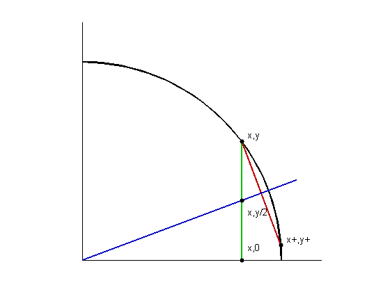
Pythagorean Addition
Blogs


Comments
To leave a comment, please click here to sign in to your MathWorks Account or create a new one.