
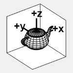
Investigate the Mathematics of Computer Graphics
Matrices in action.
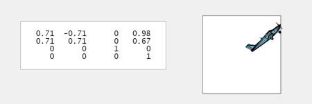
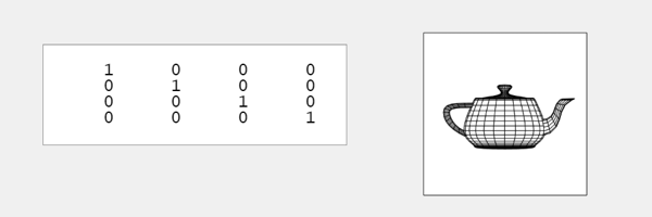
The 4-by-4 matrix in the panel on the following screenshot is at the heart of computer graphics. It describes objects moving in three-dimensional space. It is essential to MATLAB's Handle Graphics, to CAD (Computer Added Design) packages, to CGI (Computer Graphics Imagery) in films, and to most popular video games.
Contents
Rotations
The homogeneous coordinates system used by computer graphics makes it possible to describe rotations, translations and many other operations with 4-by-4 matrices. These matrices operate on vectors with the position of an object, x, y and z , in the first three components and, for now, a one as the fourth component.
Rotations are described by products of these matrices, each of which operates on only two of the first three components of a vector. For example, $R_x$ leaves x unchanged while it rotates y and z.
$$ R_x(\theta) = \left[ \begin{array}{rrrr} 1 & 0 & 0 & 0 \\ 0 & \cos{\theta} & -\sin{\theta} & 0 \\ 0 & \sin{\theta} & \cos{\theta} & 0 \\ 0 & 0 & 0 & 1 \end{array} \right] $$
$$ R_y(\theta) = \left[ \begin{array}{rrrr} \cos{\theta} & 0 & -\sin{\theta} & 0 \\ 0 & 1 & 0 & 0 \\ \sin{\theta} & 0 & \cos{\theta} & 0 \\ 0 & 0 & 0 & 1 \end{array} \right] $$
$$ R_z(\theta) = \left[ \begin{array}{rrrr} \cos{\theta} & -\sin{\theta} & 0 & 0 \\ \sin{\theta} & \cos{\theta} & 0 & 0 \\ 0 & 0 & 1 & 0 \\ 0 & 0 & 0 & 1 \end{array} \right] $$
Translations
Translations are described by matrices with values in the fourth column. For example, multiplying a vector by $T_x$ increments x.
$$ T_x(\delta) = \left[ \begin{array}{rrrr} 1 & 0 & 0 & \delta \\ 0 & 1 & 0 & 0 \\ 0 & 0 & 1 & 0 \\ 0 & 0 & 0 & 1 \end{array} \right] $$
$$ T_y(\delta) = \left[ \begin{array}{rrrr} 1 & 0 & 0 & 0 \\ 0 & 1 & 0 & \delta \\ 0 & 0 & 1 & 0 \\ 0 & 0 & 0 & 1 \end{array} \right] $$
$$ T_z(\delta) = \left[ \begin{array}{rrrr} 1 & 0 & 0 & 0 \\ 0 & 1 & 0 & 0 \\ 0 & 0 & 1 & \delta \\ 0 & 0 & 0 & 1 \end{array} \right] $$
Scalings
This matrix applies a single scaling factor to all three axes.
$$ S(\sigma) = \left[ \begin{array}{rrrr} \sigma & 0 & 0 & 0 \\ 0 & \sigma & 0 & 0 \\ 0 & 0 & \sigma & 0 \\ 0 & 0 & 0 & 1 \end{array} \right] $$
M
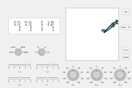
Our focus is on the matrix shown in the panel; $M$ records the product of all the transformations. The screenshots in this post show the effect of a 45 degree rotation about the z axis, followed by translations along both x and y, so $M = T_x(1.5) \, T_y(0.667) \, R_z(45)$.
grafix
Our screen shots come from our program grafix. Three dials apply rotations about the three axes; three sliders apply translations along the three axes; and one slider applies the overall scaling. Angles of rotation are specified in degrees, not radians.
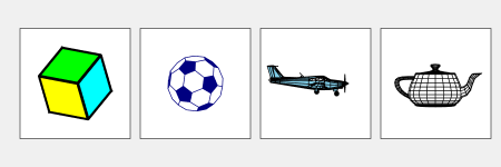
Four Objects
Choose one of four objects.
- Cube. A cube with three faces colored by the graphics primary colors, red, green and blue, and opposing faces colored by the complementary colors, cyan, magenta and yellow.
- Bucky. At first glance, this looks like a football or soccer ball, but the faces are flat. Technically, it is a trucated icosahedron. There are twelve blue pentagons and twenty white hexagons. It is the graph of the adjacency matrix of the carbon-60 atom.
- Plane. The Piper 24-250 Comanche was manufactured only between 1958 and 1972, but used models are still for sale on the Web today. Our graphics object has 97 patches and is available in the MATLAB Aerospace Toolbox.
- Teapot. The Utah teapot has been a mainstay of computer graphics since 1975. See Utah Teapot.
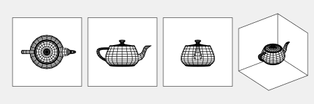
Four Views
Choose one of four static, unlit, orthogonal projection views.
- xy. The x - y plane from overhead, the positive z axis.
- xz. The x - z plane from the left side, the positive y axis.
- yz. The y - z plane from the front, the positive x axis.
- xyz. The conventional MATLAB three dimensional view.
Axis
The origin of the coordinate system is in the center of a box. One face of that box provides the background for each of the 2-D views. The three faces of that box on the opposite of the origin from the viewpoint provide the background for the 3-D view.
Programs
grafix is programmable, in a primitive sort of way. A script like this produces an animation terminating with the screen shots above.
  G = grafix('plane',0);
  for t = 0:0.1:2
      M = T_x(t-0.5) * T_y(0.333*t) * R_z(22.5*t);
      grafix(G,M)
      drawnow
  end
Software
Version 1.0 of grafix is available from this link. Everything is in a single file that can be distributed easily.
- Category:
- Color,
- Fun,
- Graphics,
- Matrices,
- Programming


See Also
-

Grafix Users Guide
Blogs
-

Rotation Matrices
Blogs
-
-
Comments
To leave a comment, please click here to sign in to your MathWorks Account or create a new one.