Function is as functiontests
Today we have a post from guest blogger Andy Campbell to highlight a function-based approach for writing tests in MATLAB. We will be demonstrating how you can write simple functions that aid you in designing a physical system. This approach allows you to iterate quickly and improve your designs while protecting you from violating requirements met by earlier solutions.
With that, let's jump right in!
Contents
Problem Statement
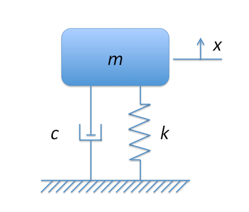
Suppose you are working on a design problem that is governed by a second order differential equation. The beauty of mathematics is that this actually has a wide range of applicability across many different areas. For our example, let's consider the design of a simple mass-spring-damper. Such a system may be used to model the suspension system on a car or truck. This is often represented using the following simplified model:

Where:
- $m$ = mass
- $k$ = spring constant
- $c$ = damping coefficient
- $x$ = displacement from equilibrium
Assuming there are no external forces, the equation of motion for this system is the solution to the second order differential equation $m\ddot{x} + c\dot{x} + kx = 0$. Following a similar approach to an earlier blog post, we can prepare this equation to be solved by one of MATLAB's ode solvers and write the following function used to evaluate our design:
type simulateSystem
function [x, t] = simulateSystem(design)

% Design variables
c = design.c;
k = design.k;

% Constant variables
z0 = [-0.1; 0];  % Initial Position and Velocity
m = 1500;        % Mass

odefun = @(t,z) [0 1; -k/m -c/m]*z;
[t, z] = ode45(odefun, [0, 3], z0);

% The first column is the position (displacement from equilibrium)
x = z(:, 1);
In this function, $z$ is a vector representing the state of the system. It contains $x$ and its derivative $\dot{x}$. Note that the initial conditions are that the mass has a position of -0.1 and its velocity is 0. This state may model the case where you are driving on the highway and hit a pothole. The initial position models the mass at the bottom of the pothole and the zero initial velocity models the suspension compressed, stopped, and about to recoil. For the sake of this example, let's say that the mass is constant at 1500 kg, which is reasonable for the load carried by a single wheel of a large light duty truck.
The design variables are the spring constant, $k$, and the damping coefficient, $c$. Initially they both have an arbitrary value of 1.
type springDamperDesign0
function design = springDamperDesign0
% Design variables
design.c = 1;          % Damping Coefficient (initial design)
design.k = 1;          % Spring Constant (initial design)
Enter functiontests
If I were tasked to design a system like this I would undoubtedly look for some requirements of the design and ensure my design meets them all. However, a problem can surface if I implement a design that fits one requirement but then adjust the design to fit a second requirement that ends up breaking the first. For one or two requirements this is fairly easy to manage but it quickly becomes intractable with many requirements or if new requirements are added at a later time. Wouldn't it be great if we had some simple mechanism to capture the first requirement to ensure it is never violated? We do! Let's write a test!
An easy way to start writing your own test function is to use the functiontests function. The functiontests function can be called at the top of your test function file, and it allows you to create and group many related tests in the same file.
type testTemplate
function tests = testTemplate

tests = functiontests(localfunctions);

end
Let's dissect what is happening here. By convention, the name of this file starts or ends with the word "test" (case insensitive) to help identify it as a function file that contains tests. All it needs to do is call the localfunctions function as input into the functiontests function, and then assign the result to the output of the main function.
What is functiontests?
functiontests is a MATLAB function (new in R2013b) that accepts a cell array of function handles to local functions within a MATLAB file. It then determines which of these local functions are tests based on naming convention and creates a Test element for each of them. All local functions that start or end with the word "test" (case insensitive) are considered tests.
What is localfunctions?
The localfunctions function is another MATLAB function that is new in R2013b. This function takes no input arguments and simply returns a cell array of handles to all of the local functions within the calling file. When testing with functiontests, using localfunctions is highly recommended so that when you add additional test functions to the file their function handles do not need to be manually added to a cell array at the top of the file. Instead, localfunctions automatically discovers these new tests and adds them to the cell array of function handles passed to functiontests.
The First Test
With this basic framework in place we can write our first test. The first design requirement might be that the system returns to equilibrium within a certain amount of time, for example, 2 seconds. Let's write a test to see how we are doing against this requirement.
type design0Test
function tests = design0Test

tests = functiontests(localfunctions);

end

function testSettlingTime(testCase)
% Test that the system settles to within 0.001 of zero under 2 seconds.

[position, time] = simulateSystem(springDamperDesign0);

positionAfterSettling = position(time > 2);

% For this example, verify the first value after the settling time.
verifyEqual(testCase, positionAfterSettling(1), 0, 'AbsTol', 0.001);
end
This test:
- Simulates the system using the specified design variables.
- Captures the position after the required settling time.
- Verifies that the position reaches 0 within +/- 0.001 by the required time. Typically for a real test you would want to verify that all positions after the settling time are sufficiently close to zero, not just the point at the desired time.
Note that this test function uses, and requires, a single testCase argument. This argument contains important test context and enables the use of a rich library of qualification functions such as verifyEqual.
What happens when we call this function?
test = design0Test;
disp(test)
  Test with properties:

                  Name: 'design0Test/testSettlingTime'
    SharedTestFixtures: []
You can see a single test was created from this function. To run this test, simply call the run function with this test as an argument.
run(test);
Running design0Test

================================================================================
Verification failed in design0Test/testSettlingTime.

    ---------------------
    Framework Diagnostic:
    ---------------------
    verifyEqual failed.
    --> NumericComparator failed.
        --> The values are not equal using "isequaln".
        --> AbsoluteTolerance failed.
            --> The value was not within absolute tolerance.

                Tolerance Definition:
                    abs(expected - actual) <= tolerance
                Tolerance Value:
                         1.000000000000000e-03

    Actual Value:
          -0.099863405108097
    Expected Value:
             0

    ------------------
    Stack Information:
    ------------------
    In H:\Documents\LOREN\MyJob\Art of MATLAB\Andy Campbell\informal test interface\design0Test.m (testSettlingTime) at 15
    In C:\Program Files\MATLAB\R2013b\toolbox\matlab\testframework\+matlab\+unittest\FunctionTestCase.m (FunctionTestCase.test) at 90
================================================================================
.
Done design0Test
__________

Failure Summary:

     Name                          Failed  Incomplete  Reason(s)
    ===========================================================================
     design0Test/testSettlingTime    X                 Failed by verification.
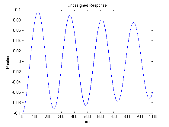
As you can see, the test failed and printed some information from verifyEqual to help diagnose the failure. Let's see how close we are graphically. Note that, for this example, in order to show the dynamics we need to show a much larger time span than our system should require. The simulateSystemOverLargeTime contains the same content as simulateSystem defined above but it has a different time span.
[x, t] = simulateSystemOverLargeTime(springDamperDesign0);
plot(t, x);
title('Undesigned Response');
xlabel('Time');
ylabel('Position')

This plot demonstrates how this design doesn't come close reaching equilibrium under 2 seconds (it is not even close after 1000 seconds). However, this is to be expected since we haven't designed anything yet.
The First Design
Assume we come up with the following design:
type springDamperDesign1
function design = springDamperDesign1
design.k = 5e6; % Spring Constant
design.c = 1e4; % Damping Coefficient
Does this design meet our criteria?
run(design1Test);
Running design1Test
.
Done design1Test
__________
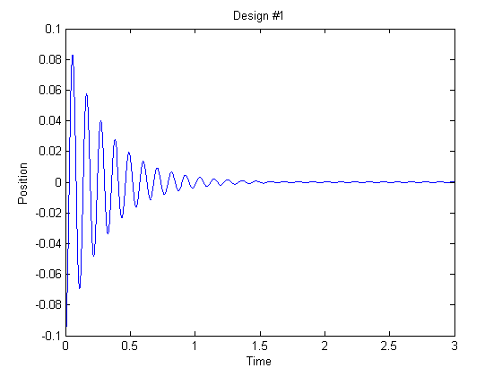
Yes it does, we've passed! Let's take a look at our response:
[x, t] = simulateSystem(springDamperDesign1);
plot(t, x)
title('Design #1')
xlabel('Time')
ylabel('Position')

Great, we reach equilibrium rapidly enough. However, unfortunately it doesn't look like a comfortable ride in your brand new truck. It looks like all the vibration from hitting a pothole will shake the poor passengers' eyes right out of their sockets. In addition, the system has overshot the equilibrium point by 80% of the pothole depth (0.08 maximum position with a pothole depth of 0.1). We can do better. Let's write a test to prove it.
The Second Test
The missing requirement here could be a restriction on how far the position can overshoot the equilibrium point. We can now add a second test to our arsenal:
type design1SecondTest
function tests = design1SecondTest

tests = functiontests(localfunctions);

end

function testSettlingTime(testCase)
% Test that the system settles to within 0.001 of zero under 2 seconds.

[position, time] = simulateSystem(springDamperDesign1);

positionAfterSettling = position(time > 2);

% For this example, verify the first value after the settling time.
verifyEqual(testCase, positionAfterSettling(1), 0, 'AbsTol', 0.001);
end

function testOvershoot(testCase)
% Test to ensure that overshoot is less than 0.01

position = simulateSystem(springDamperDesign1);
overshoot = max(position);

verifyLessThan(testCase, overshoot, 0.01);
end
This overshoot test uses verifyLessThan to ensure that the position never moves too far above the equilibrium point. We would expect this test to fail with our current design. First, we again create the Test array. Note that the second test was picked up automatically and the Test array now contains two elements instead of one.
tests = design1SecondTest;
disp(tests)
run(tests);
  1x2 Test array with properties:

    Name
    SharedTestFixtures

Running design1SecondTest
.
================================================================================
Verification failed in design1SecondTest/testOvershoot.

    ---------------------
    Framework Diagnostic:
    ---------------------
    verifyLessThan failed.
    --> The value must be less than the maximum value.

    Actual Value:
           0.082943282378938
    Maximum Value (Exclusive):
           0.010000000000000

    ------------------
    Stack Information:
    ------------------
    In H:\Documents\LOREN\MyJob\Art of MATLAB\Andy Campbell\informal test interface\design1SecondTest.m (testOvershoot) at 24
    In C:\Program Files\MATLAB\R2013b\toolbox\matlab\testframework\+matlab\+unittest\FunctionTestCase.m (FunctionTestCase.test) at 90
================================================================================
.
Done design1SecondTest
__________

Failure Summary:

     Name                             Failed  Incomplete  Reason(s)
    ==============================================================================
     design1SecondTest/testOvershoot    X                 Failed by verification.
The overshoot test fails, and this is not a bad thing! Not only does it inform us that we are missing this requirement, it also serves as a sanity check to confirm that our tests are indeed doing what we think they are doing.
The Second Design
Based on the response of the system, it seems our current design is underdamped, so why don't we just add some damping to prevent our overshoot and run the tests again.
type springDamperDesign2
function design = springDamperDesign2

design.k = 5e6;   % Spring Constant
design.c = 2.5e6; % Increase the Damping Coefficient from 1e4
Let's see how this does
[x, t] = simulateSystem(springDamperDesign2);
plot(t, x)
title('Design #2')
xlabel('Time')
ylabel('Position')

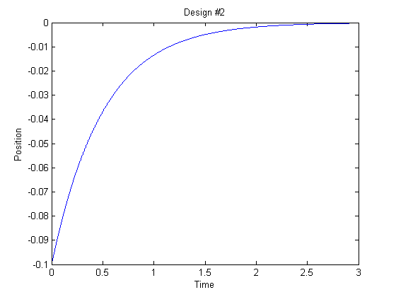
Looking at the response of this system it seems like a nice smooth ride that gently moves the truck back to equilibrium after the disturbance. Let's go with it! First let's just make sure it passes our tests.
run(design2Test);
Running design2Test

================================================================================
Verification failed in design2Test/testSettlingTime.

    ---------------------
    Framework Diagnostic:
    ---------------------
    verifyEqual failed.
    --> NumericComparator failed.
        --> The values are not equal using "isequaln".
        --> AbsoluteTolerance failed.
            --> The value was not within absolute tolerance.

                Tolerance Definition:
                    abs(expected - actual) <= tolerance
                Tolerance Value:
                         1.000000000000000e-03

    Actual Value:
          -0.001823826310161
    Expected Value:
             0

    ------------------
    Stack Information:
    ------------------
    In H:\Documents\LOREN\MyJob\Art of MATLAB\Andy Campbell\informal test interface\design2Test.m (testSettlingTime) at 15
    In C:\Program Files\MATLAB\R2013b\toolbox\matlab\testframework\+matlab\+unittest\FunctionTestCase.m (FunctionTestCase.test) at 90
================================================================================
..
Done design2Test
__________

Failure Summary:

     Name                          Failed  Incomplete  Reason(s)
    ===========================================================================
     design2Test/testSettlingTime    X                 Failed by verification.
Look at that! This design passes the overshoot test, but we have regressed and, once again, failed the settling time test. This is where we see the value in encoding these requirements through testing. There was some point after we secured the settling time requirement that we changed our focus to the overshoot requirement. It ended up being way too easy to evolve our design when tuning the overshoot and lose sight of the settling time. Focusing on overshoot, the latest design seems so reasonable, and since it is close to meeting the settling time requirement it was hard to notice through manual inspection. Obviously, close is not good enough! These tests are now protecting us from violating previously met requirements. These tests can be used to lockdown all past requirements, even when they are no longer in focus. Adding more tests can only make these requirements stricter or more complete.
This is especially important as the number of requirements for your system grows. You can become more protected by a larger and more comprehensive set of tests. You might imagine a case where you adjust the design in one way and 1 test out of 100 fails, but then you adjust the design in a different way and 75 tests out of 100 fail. When MATLAB is used to execute all of the tests in a single call you are able to gain insight into such cases, suggesting that the former design is likely closer to meeting your full set of requirements than the latter.
Since these tests use the standard MATLAB test framework they can be shared with colleagues and/or customers who can easily run them and verify that they capture the requirements sufficiently. The tests act as an executable specification of the requirements, as well as the validation that these requirements are met.
The Final Design
For completeness, let's go ahead and make this test pass and then we can debrief. With a second order system we can design for critical damping and run the tests again.
type springDamperDesign3.m
result = run(design3Test);
[x, t] = simulateSystem(springDamperDesign3);
plot(t, x)
title('Design #3')
xlabel('Time')
ylabel('Position')
function design = springDamperDesign3
m = 1500; % Need to know the mass to determine critical damping

design.k = 5e6;                   % Spring Constant
design.c = 2*m*sqrt(design.k/m);  % Damping Coefficient to be critically damped

Running design3Test
..
Done design3Test
__________

The tests pass and the response looks as expected for critical damping. Now we can move forward improving our design with the knowledge that we are protected against failing to meet our first two requirements.
Conclusion
Through a simplified example, we have demonstrated the power in using tests to validate engineering and scientific problems. All it took was writing a MATLAB function containing a couple of structured local functions. What's next? Well, for this design there might be any number of next steps, such as:
- Testing to ensure the spring constant is low enough to have a smoother, less jerky response.
- Testing to limit the cost of the springs and/or dampers (perhaps stiffer springs cost more money).
- Testing to ensure the natural frequency of the system lies within a certain range.
- Improving the model. In the real world an accurate model is likely much more complicated than a canonical second order system.
- Testing the design against a payload. For example, if the mass needs to operate with cargo with additional mass within the range of 0 to 500 kg.
- Testing the shape and characteristics of the frequency response.
The tests we wrote today are testing only the results of a given design. Remember the underlying system does not need to be a mass-spring-damper at all. The design and/or model can completely change, but these tests still are available to ensure that the response of the system meets the requirements.
The initial investment of writing a test up front yields lasting dividends and provides a safety net for analysis and design. It is interesting that these activities are what we, as scientists and engineers, already do anyway. We always test our designs, we just don't always capture the process in the form of an executable test for future execution. This approach gets easier and easier to do the more you get the hang of it. Furthermore, any time invested in such tests up front quickly pays off in productivity gains by allowing safe, rapid design iterations.
This example only begins to scratch the surface of MATLAB testing capabilities. For more information, take a look at the documentation for the MATLAB Unit Test Framework, which includes this approach using test functions. Let us know what you think here!
- Category:
- How To,
- New Feature,
- Tool


Comments
To leave a comment, please click here to sign in to your MathWorks Account or create a new one.