
Generating an Optimal Employee Work Schedule Using Integer Linear Programming
Today's guest blogger is Teja Muppirala, who is a member of our Consulting Services group. Teja has been with MathWorks for 6 years and is based in our Tokyo office.
Contents
- Mixed-Integer Linear Programming and The Nurse Scheduling Problem
- Problem Statement
- 1. Read in the requirements and employee data from the Excel sheet
- 2. Generate the f, A, and b matrices based on the the constraints and objectives
- 3. Call intlinprog with every variable as an integer 0 or 1
- 4. Gather and display the results
- 5. Conclusion
Mixed-Integer Linear Programming and The Nurse Scheduling Problem
Since it's introduction in release R2014a, we've had several blog posts now showing some applications of intlinprog , the mixed-integer linear programming (MILP) solver found in the Optimization Toolbox. This had been one of our most requested features, as MILP has trememdous application in a variety of areas such as scheduling and resource optimization.
There are a number of classic optimization problems that can be framed using MILP, such as the Travelling Salesman Problem and Knapsack Problem.
The work in this blog post is based loosely on a discussion I recently had with a customer, who wanted to make an optimal shift schedule for his employees while satisfying certain availability and staffing constraints. This is a variation of what is known as the Nurse Scheduling Problem.
Problem Statement
Obviously the "Nurse Scheduling Problem" is not limited to "nurses" as an occupation, so I will just use the generic term "employee" here. The customer's problem statement was as follows.
Given:
- A list of employees with their available work hours, and hourly salaries
- A prescibed minimum number of staff needed to be at work at a given hour (fewer staff are needed at night, more staff are needed during peak hours)
Find a schedule which MINIMIZES:
- The total daily wages the employer must pay out.
While meeting the hard CONSTRAINTS:
- At any given hour, you must meet the minimum staffing requirement
- An employee can only work one shift a day
- An employee must work within his available hours
- If an employee is called for duty, they must work at least a specified minimum number of hours, and no more than a specified maximum number of hours
This is probably a bit abstract, but let's load in some concrete data so you can get a clearer idea of what exactly we are trying to do here.
1. Read in the requirements and employee data from the Excel sheet
The staff information and scheduling requirements are in an Excel file, so we will first need to import the data. This is a fictional dataset and the Excel file is available along with the MATLAB code for this blog post so you can feel free to try it out on your own.
The first sheet in the Excel file (available here) contains the staff information, and it is in a tabular format suitable to be imported directly as a MATLAB table using the readtable function. Let's take a look at what's inside.
filename = 'scheduling.xlsx';
staffTable = readtable(filename)
staffTable =
    EmployeeName    MinHours    MaxHours    HourlyWage    Availability
    ____________    ________    ________    __________    ____________
    'SMITH'         6           8           30            '6-20'
    'JOHNSON'       6           8           50            ''
    'WILLIAMS'      6           8           30            ''
    'JONES'         6           8           30            ''
    'BROWN'         6           8           40            ''
    'DAVIS'         6           8           50            ''
    'MILLER'        6           8           45            '6-18'
    'WILSON'        6           8           30            ''
    'MOORE'         6           8           35            ''
    'TAYLOR'        6           8           40            ''
    'ANDERSON'      2           3           60            '0-6, 18-24'
    'THOMAS'        2           4           40            ''
    'JACKSON'       2           4           60            '8-16'
    'WHITE'         2           6           55            ''
    'HARRIS'        2           6           45            ''
    'MARTIN'        2           3           40            ''
    'THOMPSON'      2           5           50            '12-24'
    'GARCIA'        2           4           50            ''
    'MARTINEZ'      2           4           40            ''
    'ROBINSON'      2           5           50            ''
The variable staffTable has a list of each employee, along with the minimum hours they must work (if they are called in), maximum hours they may work, their hourly wage, and any limits on availability if there are any.
For example, the first employee SMITH, if called in, must work at least 6 hours, no more than 8 hours, earns $30/hour, and is only available between 6am and 8pm.
We can also see the required staffing requirements for each hour of the 24-hour day. I don't need this to be table, I just want to import it as a numeric array, so xlsread will work just fine.
requirements = xlsread(filename,2); % Second sheet has minimum staff requirements
disp('Required staffing (hourly from 0:00 - 24:00): ');
disp(mat2str(requirements(2,:)));
Required staffing (hourly from 0:00 - 24:00):
[1 1 2 3 6 6 7 8 9 8 8 8 7 6 6 5 5 4 4 3 2 2 2 2]
Late at night, only 1 or 2 employees are needed, while during peak hours in the morning to afternoon, we may need as many as 9 employees on duty.
2. Generate the f, A, and b matrices based on the the constraints and objectives
Generating a MILP formulation of a particular problem involves expressing the minimization objective and constraints using linear equations, and these are typically written using matrix notation. The specifics of this are covered thoroughly in the documentation.
There is a bit of machinery involved in generating the appropriate matrices in this particular case, and it would be a bit dense to go through all the details in this blog post. My aim is more to show an application of MILP, rather than discussing the intricate details of problem formulation. If you are interested in that though, I definitely encourage you to download the MATLAB files for this example and check it out for yourself.
However, I do want to discuss briefly the structure of the constraint matrices and decision variables for this particular problem. Let's take a look at the constraint matrix A. Here I used the spy function to view the sparsity pattern.
% f,A,b are inputs for the MILP Problem
% staffNumberVector is needed later when plotting the results
[f,A,b,staffNumberVector] = makeMILPMatrices(staffTable,requirements);

figure,
spy(A,1); axis fill;
title({'Sparsity pattern of the constraint matrix A:';
       'The top portion is from the minimum hour requirement,';
       'The bottom portion is from the one-shift-a-day requirement'});
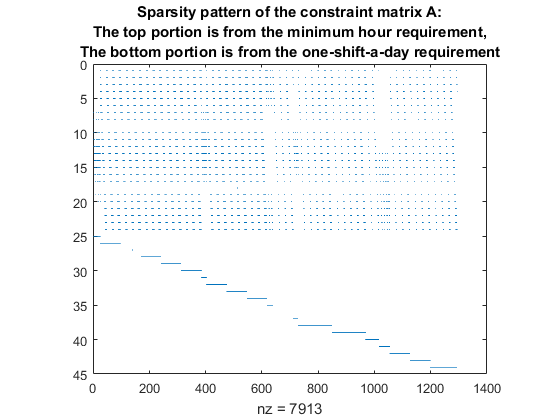
There are two parts to the inequality constraint matrix A, which are clearly visible. The top portion has 24 rows (because there are 24 hours in a day) and each row represents the constraint that at a particular hour, you need a minimum number of staff.
The bottom section of A, in this case, has 20 rows (because there are 20 available employees). The k-th row of this section is associated with the constraint that the k-th employee may only work one shift per day.
A will in general be much wider than tall, and the columns of A represent every possible shift for every possible employee. Every column of A is also associated with a decision variable that we constrain to be either 0 or 1 (a binary variable).
$\textbf{x} = [x_1,x_2,...x_k]$
${x_n} \in \{0,1\}$ for all n
A value of 1 for $x_n$ means that that n-th shift possibility is implemented, and a value of 0 indicates it is not. For this particular problem, A has 1295 columns, and so x is a decision vector of length k = 1295. It is this x that intlinprog will solve for.
As the number of employees and possible shifts increases, A may consist of many thousands of columns. Although I didn't use sparse matrices in this demo, intlinprog is capable of working with sparse matrices to make more efficient use of memory and allow for larger problem sizes.
3. Call intlinprog with every variable as an integer 0 or 1
Once the relevant matrices are created, all that's left to do is actually call intlinprog. I specify that all the decision variables are integers, and have a value between 0 and 1.
nVars = numel(f);  % Number of variables in the problem
lb = zeros(nVars,1);    % The upper and lower bounds are 0 and 1
ub = ones(nVars,1);
[x, cost] = intlinprog(f,1:nVars,A,b,[],[],lb,ub);
LP:                Optimal objective value is 4670.000000.

Cut Generation:    Applied 1 zero-half cut.
                   Lower bound is 4670.000000.

Branch and Bound:

   nodes     total   num int        integer       relative
explored  time (s)  solution           fval        gap (%)
      49      0.07         1   4.670000e+03   0.000000e+00

Optimal solution found.

Intlinprog stopped because the objective value is within a gap tolerance of the
optimal value, options.TolGapAbs = 0 (the default value). The intcon variables
are integer within tolerance, options.TolInteger = 1e-05 (the default value).
I am returning two arguments, the first is the decision vector itself, x, and the second argument, cost, is the minimized daily cost associated with this solution. You could also find cost as
cost = f*x.
intlinprog by default outputs certain diagnostic information to the command window (though there are options to hide this if preferred). For example, the miminized cost is shown in the command window to be 4670.0 (in real-world terms, $4760 dollars in daily wages). Also, one can see the total time that it took to solve this problem.
intlinprog is very fast!
4. Gather and display the results
intlinprog will give me my optimal x vector, but this is simply a long vector of of ones and zeros saying which shifts are implemented. I will go back and find out which index of x corresponds with which employee and shift, and then display the data in a more human-friendly form.
numStaff = size(staffTable,1); % Total number of staff available

% Convert from indices in x to employee and shift information
selected = find(x);
hoursMatrix = zeros(numStaff,24);

for n = 1:numel(selected);
    thisEntry =selected(n);
    thisStaff = staffNumberVector(thisEntry);
    hoursOnDuty = -A(1:24,thisEntry);
    hoursMatrix(thisStaff,:) = hoursOnDuty;
end

% Make a figure in a suitable location
hf = figure('visible','off','units','pixel','position',[100 100 560 700]);
movegui(hf,'center');
set(hf,'visible','on');

% Draw the employee work schedule matrix
subplot(211);
imagesc(0.5:23.5,1:20,hoursMatrix)
set(gca,'xtick',0:24);
set(gca,'ytick',1:numStaff,'yticklabel',staffTable.EmployeeName);
axis tight;
set(gca,'xlimmode','manual','ylimmode','manual','layer','bottom');
hold all;
ylabel('Employee Name','FontSize',12);

% Let's make the grid lines manually...
for n = 0.5:numStaff+0.5
    plot(xlim,[n n],'k');
end
for n = 0:24
    plot([n n], ylim,'k');
end

title(['Employee shift schedule' 10 ...
       'Total wages over 24 hours: $' num2str(cost)],'FontSize',16);
colormap([1 1 1; 0 0.5 1]);

% Draw the required vs. actual staff
subplot(212);
plot(0.5:23.5,requirements(2,:),'b.-','linewidth',3,'markersize',30);
actualHours = -A(1:24,:)*x;
hold on;
plot(0.5:23.5,actualHours,'r:.','linewidth',2,'markersize',16);
xlim([0 24]);
set(gca,'xtick',0:24,'ytick',0:10);
ylim([0 10]);
grid on;
title(['Hourly Staff Count'],'FontSize',16);
legend({'Employees Required', 'Employees Scheduled'});
xlabel('Time of day','fontsize',12);
ylabel('Employee count','fontsize',12);

We have two plots here. The first shows the actual work schedule for each employee (blue indicates when on shift). Note that there are a couple of employees (ANDERSON and JACKSON) that do not get called in. Also, while it seems that JOHNSON has two shifts, this is because we are wrapping around and the shift actually goes from 10pm to 6am the next morning.
The second plot shows the number of staff on duty as compared to our minimum staffing requirements. We see that we meet the requirements exactly, without overstaffing or understaffing at any point. This makes sense, because if the goal is to minimize paid wages, then you'd try to stay as close to the minimum staff as possible.
5. Conclusion
The problem outlined in the example is not a trivial one to solve. To be sure, it takes a bit of study and experience to be able to know how to easily convert a real world problem into its equivalent MILP formulation.
But for problems like this, especially at larger problem sizes, attempting to solve it using other methods such trial-and-error or genetic algorithms will usually take longer, and generally not yield as good results.
Have you tried using MATLAB's mixed-integer linear programming solver for any of your own work? If you want to share your thoughts, or if you have any questions regarding this example, please feel free to let us know in here.


Comments
To leave a comment, please click here to sign in to your MathWorks Account or create a new one.